Chapter 2 Measuring Petrophysical Properties

The measurement of petrophysical properties is performed through specialized laboratory experiments, which in the petroleum industry are classified as routine or special core analysis (SCAL), depending on the experiment complexity and on its investigated properties.

The analyzed rock samples may be extracted from well cores or from open borehole sidewall sampling tools, and can measure from one to several centimeters (Kennedy 2015). The rock samples are commonly extracted as cylindrical plugs, but can also have irregular shapes, case in which they are referred to as rock fragments.

2.1 Routine Core Analysis

Experimental measurements of a rock sample pore volume \(V_p\), grain volume \(V_g\), porosity \(\phi\) and absolute permeability \(k_{abs}\) are commonly referred to as routine core analysis.

Porous media can be pictorially described as being constituted of grain and pore spaces (Figure 2.1). The percentage of the total space occupied by pores is known as rock porosity. \(V_p\) and \(\phi\) measurements are important for the evaluation of hydrocarbon reserve volumes.

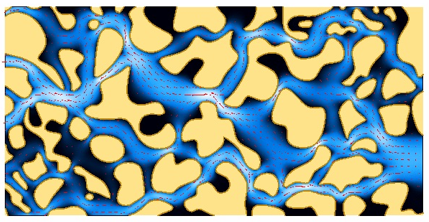
Figure 2.1: Pore media grain and pore spaces

\[\begin{equation} \phi = \frac{V_p}{V_p + V_g} \tag{2.1} \end{equation}\]

At reservoir conditions, porous space is filled by either water, oil or gas, each of which in a separate phase. The percentage of the porous volume occupied by water, oil or gas is known as water, oil or gas saturation, respectively.

\[\begin{equation} S_f = \frac{V_f}{V_p},\quad \text{for} \;f \; \text{in} \; {w, o, g} \tag{2.2} \end{equation}\]

Darcy’s law (2.3) describes the linear relationship between instantaneous flow rate \(q\) and a pressure gradient \(\frac{\partial p}{\partial x}\) in laminar single-phase flow (Tiab and Donaldson 2004). Given a stable steady-state single-phase flow, the porous media absolute permeability \(k_{abs}\) is directly proportional to the instantaneous flow rate \(q\), fluid viscosity \(\mu\), and is inversely proportional to the pressure gradient \(\frac{\partial p}{\partial x}\) and cross-sectional area \(A\).

\[\begin{equation} q = k_{abs}\frac{A}{\mu}\frac{\partial p}{\partial x} \tag{2.3} \end{equation}\]

2.2 Special Core Analysis

Measurement of multiphase properties of porous media, on which both viscous and capillary forces may be relevant, is usually more complex and incurs in longer and costlier experiments when compared to single-phase routine core analysis measurements.

2.2.1 Mercury Injection Capillary Pressure

In multi-phase porous systems, due to different interaction characteristics between fluid and solid phases, the attraction between the molecules of one of the fluid phases and the solid surfaces may be greater than that of the other fluid phase. This physical behavior is known as wettability, and it is responsible for capillary forces and related phenomena.

For a given multiphase porous system, with a surface tension \(\sigma\) between fluid phases, wettability may be quantified by the contact angle \(\theta\) formed by the fluid phase boundary-solid interface, as depicted in Figure 2.2.

The Young-Laplace equation describes the capillary pressure sustained across the interface between fluids at a pore throat constriction (Tiab and Donaldson 2004). A heterogeneous porous system is connected by pore throats of several different radii. For a system consisting of mercury and mercury vapor, with surface tension \(\sigma_{Hg-air}\) and contact angle \(\theta_{Hg-air}\) with the rock surface, the relationship between capillary pressure and pore throat radius r may be described by equation (2.4). Capillary forces may strongly affect the distribution of fluid phases in the porous space.

Figure 2.2: Contact Angle between fluid phase boundary and solid surface

\[\begin{equation} P_c = \frac{2\sigma_{Hg-air} \cos{\theta_{Hg-air}}}{r} \tag{2.4} \end{equation}\]

A Mercury Injection Capillary Pressure (MICP) experiment consists of pre-specified and controlled mercury injection steps in a porous medium, previously subjected to a vacuum. It is usually performed on rock fragments with around one cubic centimeter, which allows it to be executed both in well core and sidewall sample fragments. Automated acquisition systems for MICP are commercially available (Micromeritics 2020)(Figure 2.3), making it a relatively fast and cheap experiment.

A fixed pressure stabilization time and a geometric progression sequence of increasing pressure steps is defined before each MICP experiment. At each pressure step, after the pre-defined pressure stabilization time, the volume of intruded mercury in the rock sample pore space is recorded. Given calibrated mercury-mercury-vapor surface tension \(\sigma_{hg-air}\) and contact angle \(\theta_{hg-air}\), each pressure step may be associated with a pore throat radius according to equation (2.4). The cumulative intruded mercury volume \(V_{hg}\) at each step, thus, corresponds to the porous volume accessible by pore throats with radius equal to or smaller than the relationship given by equation (2.4). Mercury saturation \(S_{hg}\) at each step may be calculated using equation (2.5).

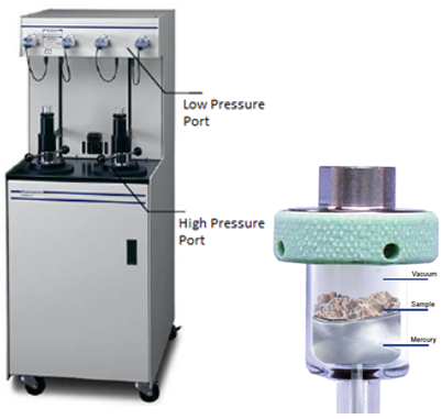
Figure 2.3: AutoPore IV Series Mercury Porosimeter (left) and glass penetrometer (right) used in automated MICP acquisitions.

\[\begin{equation} S_{hg} = \frac{V_{hg}}{V_T} \tag{2.5} \end{equation}\]

The total fragment volume \(V_T\) is estimated during the experimental data interpretation procedure, using the difference of the total glass bulb volume and the intruded mercury volume necessary to “envelope” the rock fragment and start intruding the porous space. This happens at a pressure known as entrance capillary pressure \(P_e\) The determination of the exact value of this entrance capillary pressure may introduce uncertainty on experimental results, particularly for very irregular shaped or vuggy rock samples.

The recorded capillary pressure \(P_c\) and mercury saturation \(S_{hg}\) values form a capillary pressure curve, whose format is directly related to the distribution of accessible pore volume in the porous medium of the rock sample. Figure 2.4 shows several capillary pressure curves acquired in MICP experiments.

A widely used transformation of capillary pressure curves is described by equation (2.6) (Lenormand 2003), which constructs a probability distribution of accessible pore volume as a function of the logarithm of the associated pore throat radius \(r\). Figure 2.5 shows pore volume probability distribution curves \(p(\log{r})\), for the same MICP experiments depicted in Figure 2.4.

\[\begin{equation} p(\log{r}) = \frac{dS_{hg}}{d \log{P_c}} \tag{2.6} \end{equation}\]

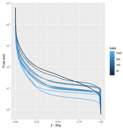
Figure 2.4: Mercury Injection Capillary Pressure Curves for several rock samples, colored by absolute permeability.

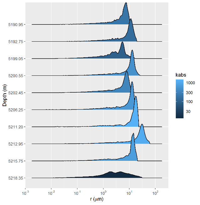
Figure 2.5: Accessible pore volume probability distribution curves p(log r), for the same MICP experiments depicted in Figure 2.4.

Several authors have proposed correlations between capillary pressure curve features and absolute permeability (Kolodzie 1980; Pittman 1992; Purcell 1949; Swanson 1981), among others. These correlations will be further explorer on chapter .

In this work, a dataset of 2324 MICP curves acquired on rock fragments of sandstone and carbonate reservoirs from several Brazilian reservoirs was compiled. Routine and special core analysis results, performed on core sample plugs and sidewall samples extracted from the same well depths as the rock fragments were incorporated in the dataset.

Given that the size of the rock fragments utilized for MICP measurements were in many cases many times smaller than the size of the corresponding core sample plugs and sidewall samples, where routine and special core analysis were performed, it is very likely that, for many samples, the rock fragments may not constitute a representative volume of the porous space (Blunt 2017). Indeed, as illustrated in Figure 2.6, it is possible to assess that heterogeneous reservoirs display many more outlier samples on correlations between MICP and core analysis data, when compared to more homogeneous reservoirs.

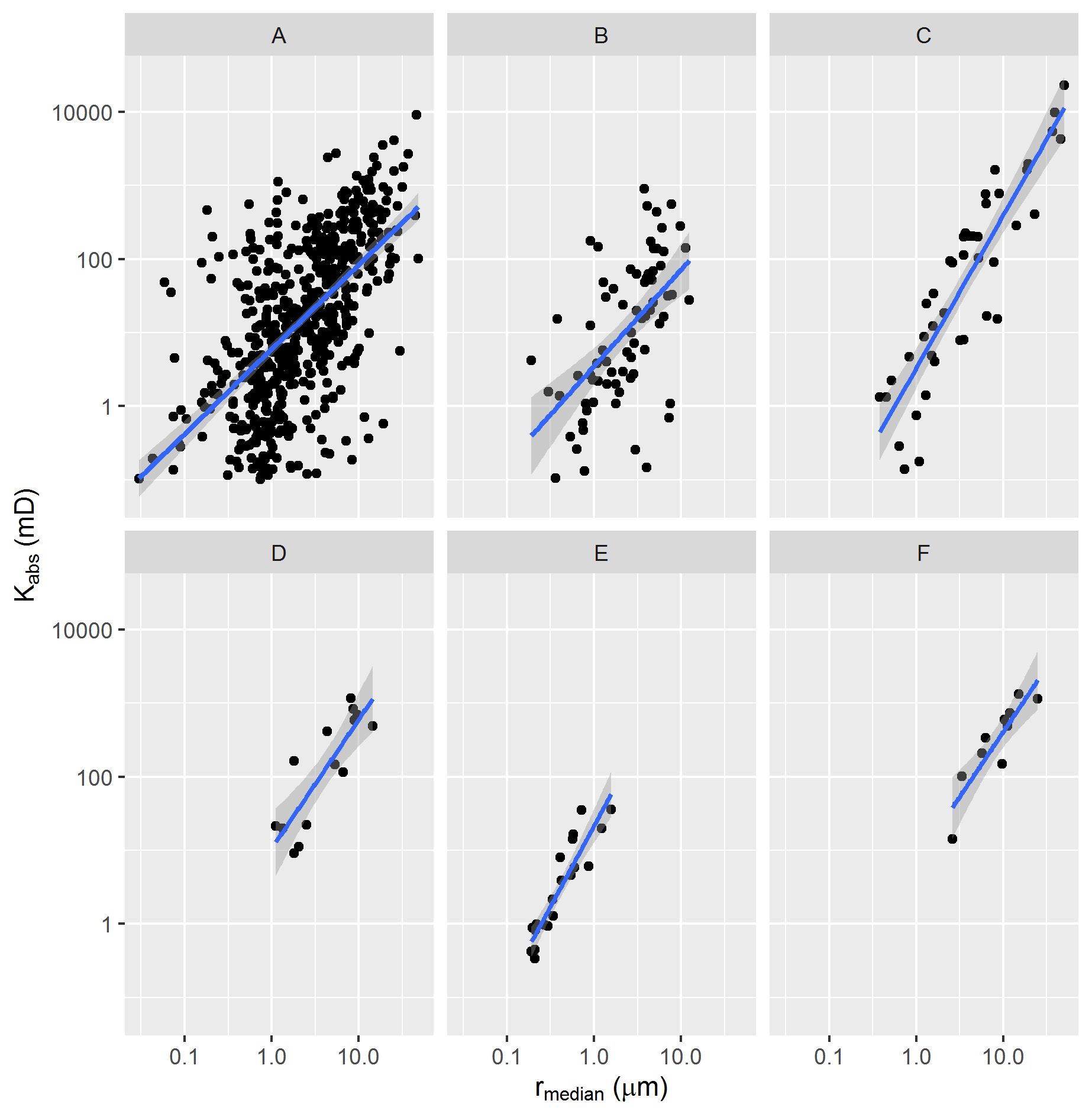
Figure 2.6: Relationship between median pore throat radius and absolute permeability of several different reservoirs, from most to least heterogeneous

2.2.2 Centrifuge Capillary Pressure

The centrifuge method is a standard technique for capillary pressure curve estimation of porous media. The method consists of imposing a capillary pressure profile on a rotating rock sample through centrifugal acceleration imposition in increasing rotation speed steps, and recording the average sample saturation at each step (Tiab and Donaldson 2004). The fundamental equations that describe the method were developed by Hassler and Brunner (Hassler and Brunner 1945):

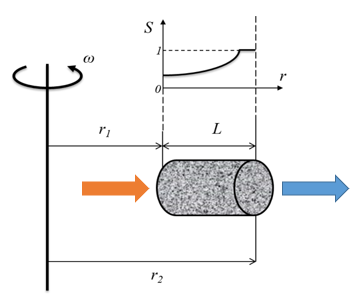
Figure 2.7: Drainage Oil-Water Centrifuge capillary pressure experiment geometry.

\[\begin{equation} P_c = \frac{1}{2}\omega^2\Delta \rho (r^2-r_{2}^{2}) \tag{2.7} \end{equation}\]

\[\begin{equation} B = 1 - (\frac{r_1}{r_2})^2 \tag{2.8} \end{equation}\]

\[\begin{equation} S_w = \frac{V_w}{V_p} = \frac{V_w}{V_w + V_o} \tag{2.9} \end{equation}\]

\[\begin{equation} \overline{S_w}(P_c)=\frac{(1+\sqrt{1-B})}{2}\int_0^1{\frac{S_w(xP_c)}{\sqrt{1-Bx}}} dx \tag{2.10} \end{equation}\]

where \(\omega\) is the centrifuge rotation speed, \(\Delta \rho\) is the difference in density between the displacing and displaced fluids, \(L\) is the rock sample length, \(r\) is the radius to the centrifuge rotation center, \(r_1\) and \(r_2\) are the radial distances to the sample extremities, \(V_p\), \(V_w\) and \(V_o\) are the sample pore, water and oil volumes, \(S_w (P_c)\) is the water saturation at a given point in the sample subjected to a \(P_c\) capillary pressure, and \(\overline{S_w}\) is the sample average water saturation.

Several methods have been proposed for the estimation of capillary pressure curves from centrifuge experiments. These methods may be classified as direct or inverse according to how they solve the centrifuge saturation equation. Direct methods use several proposed differential and integral approximations of the saturation equation to directly estimate capillary-pressure curves from centrifuge experiment measurements at discrete capillary-pressure steps (Forbes 1994; Hassler and Brunner 1945; Skuse, Flroozabadl, and Ramey Jr. 1992). Inverse methods parameterize capillary-pressure curves and solve the saturation equation using non-linear regression (Bentsen 1977) or linear regression with spline basis functions (Nordtvedt and Kolltvelt 1991).

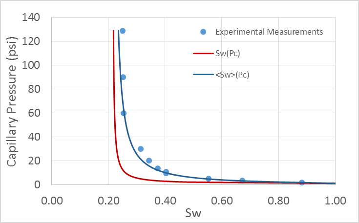
Figure 2.8: Estimation of capillary pressure curve from centrifuge measurements.

In this work, a dataset of 135 capillary pressure curves estimated from centrifuge experiments was compiled. Using the parameterization (2.11), proposed in (Albuquerque et al. 2018), each of the capillary pressure curves was fitted using a least-squares minimization procedure, with parameters \(S_{wi}\), \(P_e\), \(\alpha\) and \(\beta\).

\[\begin{equation} S_w(P_c, S_{wi}, \alpha, \beta, P_w) = \frac{1+\alpha S_{wi}(P_c - P_e)^\beta}{1+\alpha (P_c - P_e)^\beta} \tag{2.11} \end{equation}\]

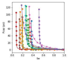
Figure 2.9: Sample of the experimental capillary pressure curve dataset (points) and fitted capillary pressure model (lines).

This parameterization is such that for high values of capillary pressure, water saturation \(S_w\) approaches \(S_{wi}\), a parameter thus named irreducible water saturation. In a drainage capillary pressure model, the smallest pressure at which the saturation of the sample can be reduced from one hundred per cent is termed “entrance” capillary pressure (Peters 2012), modeled by parameter \(P_e\) in equation (2.11). The remainder parameters \(\alpha\) and \(\beta\) are associated with the capillary pressure curve steepness and shape.

\[\begin{equation} \lim_{P_c \to +\infty} S_w = S_{wi} \tag{2.12} \end{equation}\]

\[\begin{equation} P_c(S_{w}=1) = P_e \tag{2.13} \end{equation}\]

Considering a transformation analogous to the one utilized for mercury injection capillary pressure curves (2.6), pore volume probability distribution curves \(p(\log r)\) may be estimated from the fitted centrifuge capillary pressure curve parameters, as described by equation (2.14).

\[\begin{equation} p(\log r) = \frac{dS_w}{d \log{P_c}} = \frac{\alpha \beta S_{wi} (S_w - S_{wi})(P_c - P_e)^{\beta - 1}}{1 + \alpha (P_c - P_e)^\beta} \tag{2.14} \end{equation}\]

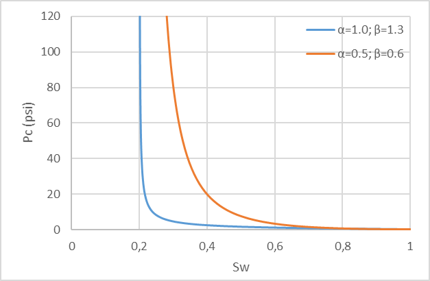
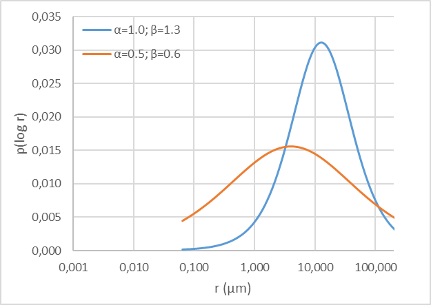
Figure 2.10: Sample centrifuge capillary pressure curves, parameterized by equation (2.11), and corresponding pore volume probability distribution curves p(log r).

As graphically displayed in Figure 2.10, the parameter \(\alpha\) can be shown to be associated with the location of the distribution \(p(\log{r})\) and the parameter \(\beta\) can be shown to be associated with its scale or dispersion.

A dataset combining the fitted centrifuge capillary pressure curve parameters and several MICP features, detailed on chapter , of rock fragments extracted from corresponding core locations was assembled. As exemplified in Figure 2.11, associated pore volume distributions of corresponding centrifuge capillary pressure and MICP curves often display similar distributions, though to varying degrees as MICP curves may have been measured in rock fragments which may or may not be representative of its associated core sample pore volume. MICP experiments also cover a larger range of pore throat radius sizes and display significantly more detail, as a much tighter pressure and corresponding pore throat radius experimental grid is sampled.

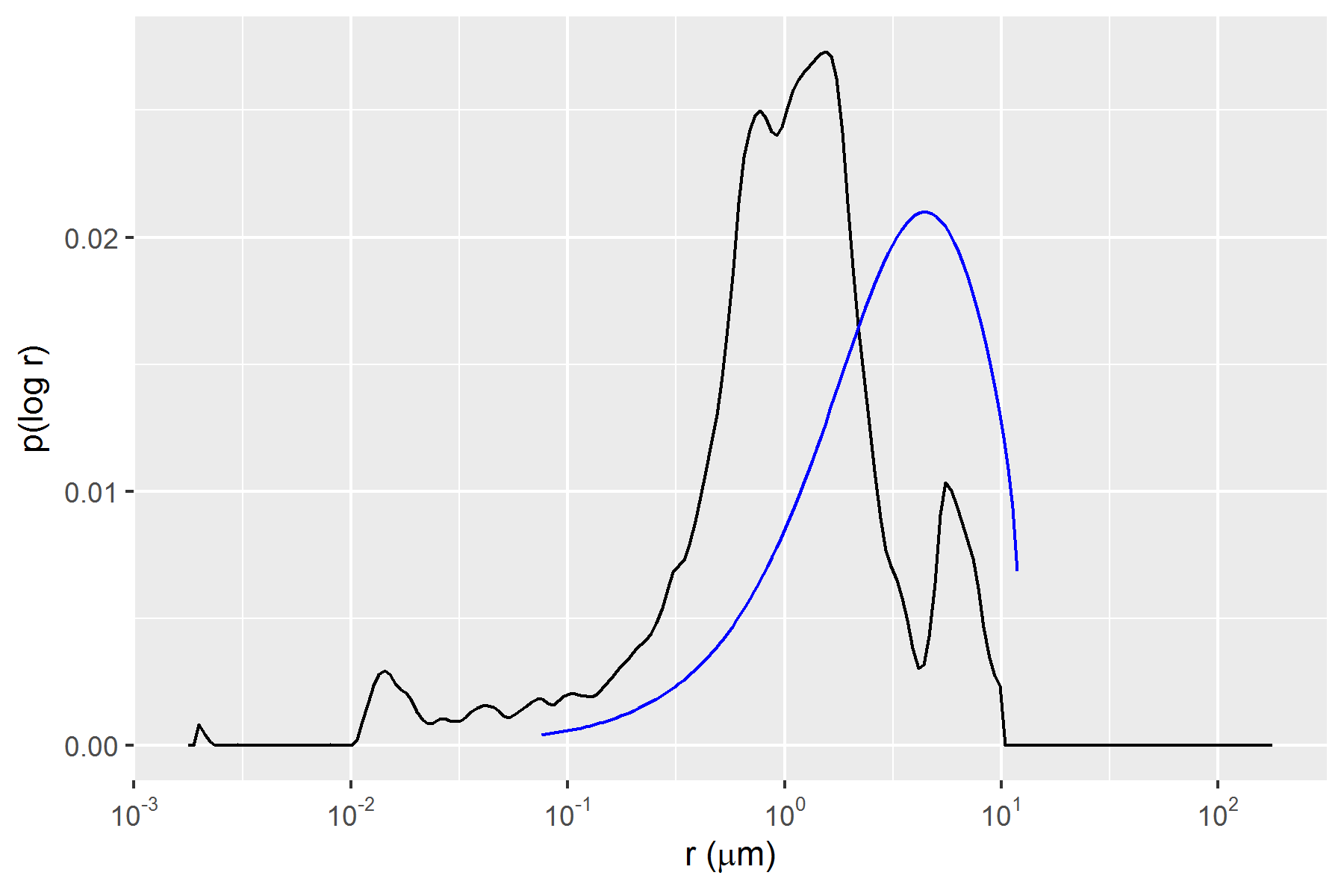
Figure 2.11: Associated pore volume distributions p(log r) of correspondent Centrifuge Capillary Pressure (blue curve) and MICP (black curve) samples.

In Figure 2.12, it is possible to identify significant correlations between corresponding centrifuge capillary pressure curves \(\alpha\), \(S_{wi}\) and MICP median pore throat radius \(r_{median}\) parameters. Both \(\alpha\) and \(S_{wi}\) parameters can be seen, thus, as correlated with the location of the distribution \(p(\log{r})\).

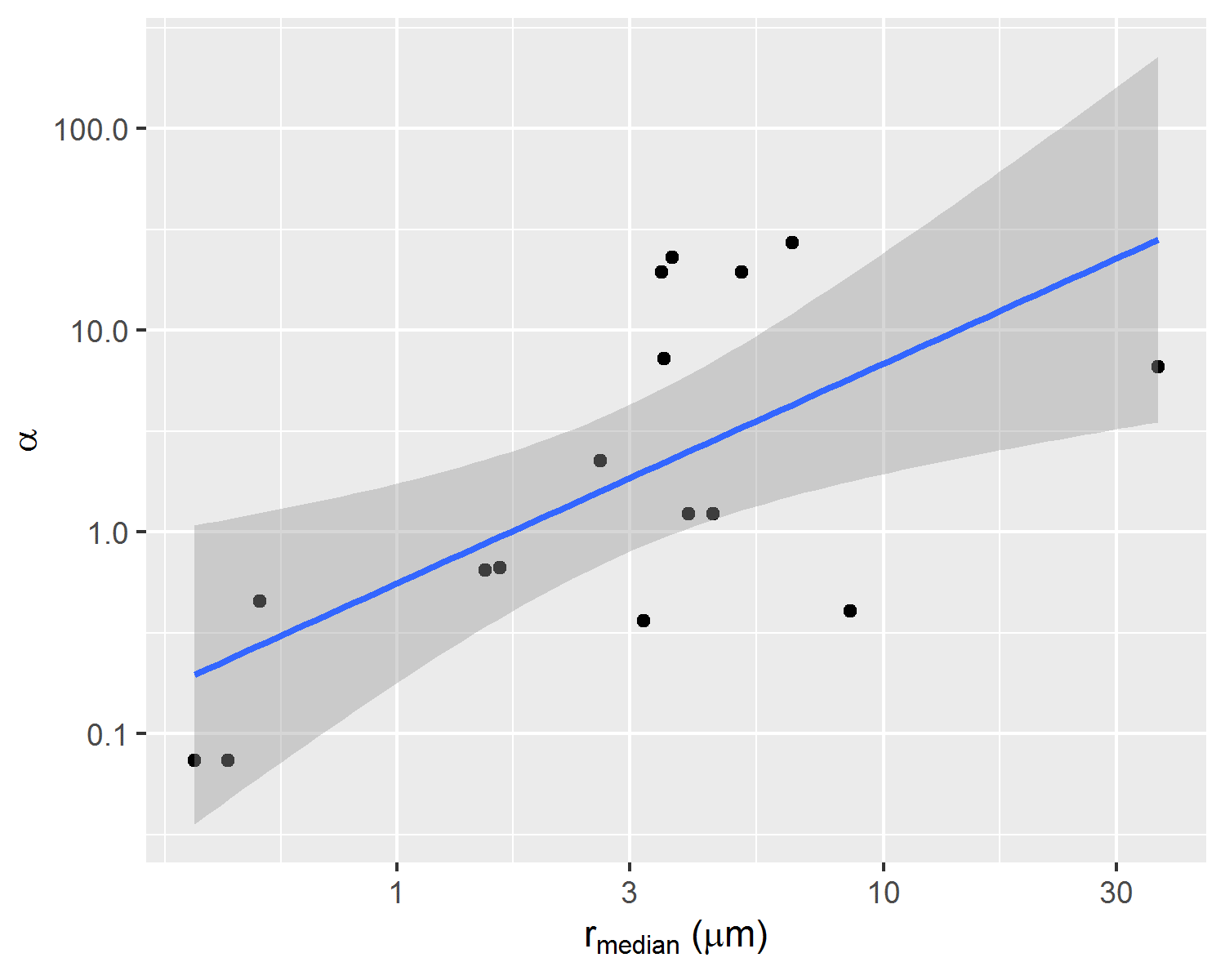
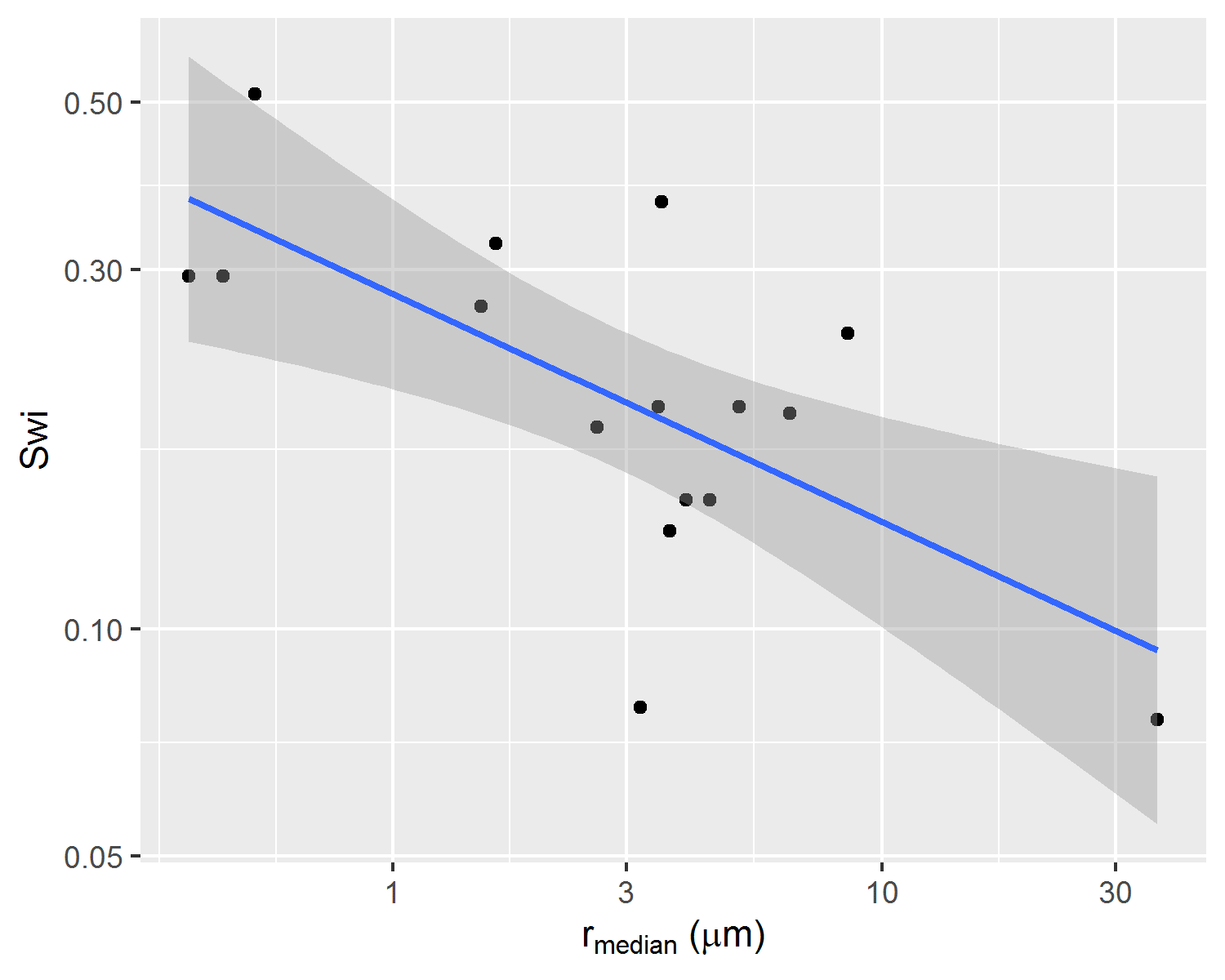
Figure 2.12: Correlations between parameters alpha, Swi and median pore throat radius of correspondent rock fragment p(log r) distribution.

2.2.3 Relative Permeability

In porous media multiphase flow, relative permeability describes the linear proportion by which each fluid flow is penalized when compared to Darcy’s law (2.3). For a water-oil two-phase flow, the following relations describe oil (\(k_{ro}\)) and water (\(k_{rw}\)) relative permeability, and the their associated fractionary water flow (\(f_{w}\)).

\[\begin{equation} q_o(S_w) = k_{ro}(S_w) \frac{k_{abs}A}{\mu_o L} \Delta p \tag{2.15} \end{equation}\]

\[\begin{equation} q_w(S_w) = k_{rw}(S_w) \frac{k_{abs}A}{\mu_w L} \Delta p \tag{2.16} \end{equation}\]

\[\begin{equation} f_w = \frac{\frac{k_{rw}}{\mu_w}}{\frac{k_{rw}}{\mu_w} + \frac{k_{ro}}{\mu_o}} \tag{2.17} \end{equation}\]

The most widely used experimental setup for water-oil relative permeability determination is the unsteady-state water-oil relative permeability experiment. In a unsteady-state water-oil relative permeability experiment, a sample initially satured at irreducible water saturation \(S_{wi}\) condition is subjected to a constant rate water injection, simulating reservoir secondary recovery water injection.

During the experiment, water injection flow rate \(q_{w_{inj}}\) and exit pressure \(P_{out}\) are kept constant, and cumulative oil production \(N_p\) and pressure differential \(\Delta p\) are recorded.

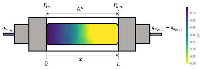
Figure 2.13: Unsteady-state relative permeability experimental setup.

\[\begin{equation} q_{w_{inj}} = cte \tag{2.18} \end{equation}\]

\[\begin{equation} P_{out} = cte \tag{2.19} \end{equation}\]

Unsteady state water-oil relative permeability experiments are usually interpreted using either the JBN method (Johnson, Bossler, and Naumann 1959) or using history matched numerical simulated solutions (Lenormand and Lenormand 2016). Figure 2.14 displays an example of recorded and history matched cumulative oil production \(N_p\) and pressure differential \(\Delta p\), obtained using maximum likelihood estimation of the relative permeability parameters that best fit the recorded experimental data.

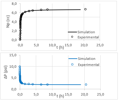
Figure 2.14: Example of history matched experimental data.

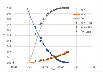
Figure 2.15: Example of history matched relative permeability and fractionary flow curves compared to analytic JBN interpreted experimental results.

History matching is usually performed using parametric relative permeability models and finite difference partial differential equations simulation. The Corey model (Corey 1954), given by equations (2.20)(2.21)(2.22), is a widely used power-law model for relative permeability curves, whose parameters \(n_o\) and \(n_w\) are commonly referred to as Corey exponents.

\[\begin{equation} S_{wD} = \frac{S_w - S_{wi}}{1 - S_{wi} - S_{or}} \tag{2.20} \end{equation}\]

\[\begin{equation} k_{ro}(S_w) = k_{ro@S_{wi}}(1-S_{wD})^{n_o} \tag{2.21} \end{equation}\]

\[\begin{equation} k_{rw}(S_w) = k_{rw@S_{or}}(S_{wD})^{n_w} \tag{2.22} \end{equation}\]

The LET model (Lomeland, Ebeltoft, and Thomas 2005), given by equations (2.23)(2.24), was developed with six shape parameters \(L_o\), \(E_o\), \(T_o\), \(L_w\), \(E_w\), \(T_w\), and can accommodate much more flexible relative permeability curves. It is commonly used in reservoir simulation models, especially for history matching procedures that demand flexible representations of relative permeability models.

\[\begin{equation} k_{ro}(S_w) = k_{ro@S_{wi}}\frac{(1-S_{wD})^{L_o}}{(1-S_{wD})^{L_o} + E_o(S_{wD})^{T_o}} \tag{2.23} \end{equation}\]

\[\begin{equation} k_{rw}(S_w) = k_{rw@S_{or}}\frac{(S_{wD})^{L_w}}{(S_{wD})^{L_w} + E_w(1-S_{wD})^{T_w}} \tag{2.24} \end{equation}\]

In this work, a dataset of 226 unsteady-state water-oil relative permeability curves was assembled. LET parameters for each of the 226 curves were fit using maximum likelihood estimation (DeGroot and Schervish 2012). Multivariate and multi-task linear regression models built using this dataset are described on chapter .

References

Albuquerque, Marcelo R, Felipe M Eler, Heitor V R Camargo, André Compan, Dario Cruz, and Carlos Pedreira. 2018. “Estimation of Capillary Pressure Curves from Centrifuge Measurements using Inverse Methods.” Rio Oil & Gas Expo and Conference 2018,

Bentsen, R G. 1977. “Using Parameter-Estimation Techniques To Convert Centrifuge Data Into a Capillary-Pressure Curve.” Society of Petroleum Engineers Journal 17 (1): 57–64. https://doi.org/10.2118/5026-PA.

Blunt, Martin J. 2017. Multiphase Flow in Porous Media: A Pore-Scale Perspective. Cambridge University Press.

Corey, A. T. 1954. “The Interrelation Between Gas and Oil Relative Permeabilities.” Producers Monthly 38-41.

DeGroot, Morris H., and Mark J. Schervish. 2012. Probability and Statistics. Edited by Addison-Wesley.

Forbes, P. 1994. “Simple and Accurate Methods for Converting Centrifuge Data Into Drainage and Imbibition Capillary Pressure Curves.” The Log Analyst.

Hassler, G. L., and E. Brunner. 1945. “Measurement of Capillary Pressures in Small Core Samples.” Petroleum Transactions of AIME 160 (1): 114–23. https://doi.org/10.2118/945114-G.

Johnson, E. F., D. P. Bossler, and V. O. Naumann. 1959. “Calculation of Relative Permeability from Displacement Experiments.” Trans. AIME.

Kennedy, Martin. 2015. Practical Petrophysics. Vol. 62.

Kolodzie, Stanley. 1980. “Analysis of Pore Throat Size and Use of the Waxman-Smits Equation to Determine Ooip in Spindle Field, Colorado.” In SPE Annual Technical Conference and Exhibition, 10. Dallas, Texas: Society of Petroleum Engineers. https://doi.org/10.2118/9382-MS.

Lenormand, R. 2003. “Interpretation of mercury injection curves to derive pore size distribution.” International Symposium of the Society of Core Analysts Internatio: SCA2003–52. https://doi.org/SCA2003-52.

Lenormand, Roland, and Guillaume Lenormand. 2016. “Recommended Procedure for Determination of Relative Permeabilities.” International Symposium of the Society of Core Analysts, 1–12. https://www.scaweb.org/wp-content/uploads/SCA-2016-Technical-Papers-Tuesday.pdf.

Lomeland, Frode, Einar Ebeltoft, and Wibeke Hammervold Thomas. 2005. “A new versatile relative permeability correlation.” International Symposium of the Society of Core Analysts, Toronto, Canada, 1–12.

Micromeritics. 2020. “AutoPore IV Series: Automated Mercury Porosimeters.” https://www.micromeritics.com/product-showcase/autopore-iv.aspx.

Nordtvedt, JE, and K Kolltvelt. 1991. “Capillary pressure curves from centrifuge data by use of spline functions.” SPE Reservoir Engineering, no. November: 497–501. https://doi.org/10.2118/19019-PA.

Peters, E. J. 2012. Advanced Petrophysics. Austin: Live Oak Book Company.

Pittman, E. D. 1992. “Relationship of porosity and permeability to various parameters derived from mercury injection-capillary pressure curves for sandstone.” https://doi.org/10.1017/CBO9781107415324.004.

Purcell, W. R. 1949. “Capillary Pressures - Their Measurement Using Mercury and the Calculation of Permeability Therefrom.” Journal of Petroleum Technology 1 (02): 39–48. https://doi.org/10.2118/949039-G.

Skuse, Brian, Abbas Flroozabadl, and Henry J Ramey Jr. 1992. “Computation and Interpretation of Capillary Pressure From a Centrifuge.” https://doi.org/10.2118/18297-PA.

Swanson, B. F. 1981. “A Simple Correlation Between Permeabilities and Mercury Capillary Pressures.” Journal of Petroleum Technology 33 (12): 2498–2504. https://doi.org/10.2118/8234-PA.

Tiab, Djebbar, and E. C. Donaldson. 2004. Petrophysics: theory and practice of measuring reservoir rock and fluid transport properties. Boston: Golf Professional Pub.