Chapter 3 Absolute Permeability Regression
Several authors have studied the use of MICP curves to estimate absolute permeability. Many of the proposed regression models use linear correlations between the logarithm of absolute permeability \(\log{k_{abs}}\) and many different proposed capillary pressure curve features (Kolodzie 1980; Pittman 1992; Purcell 1949; Swanson 1981).
Comparison of linear regression and machine learning models for the estimation of absolute permeability using MICP data has been performed on datasets from middle-east reservoirs by several authors (Al Khalifah, Glover, and Lorinczi 2020; Nooruddin, Anifowose, and Abdulraheem 2013), showing promising results for non-linear machine learning models.
In this work, a comparison of linear regression and machine learning models for the estimation of absolute permeability using MICP data is performed on a dataset of 2324 MICP curves acquired on rock fragments of sandstone and carbonate reservoirs from several Brazilian reservoirs.
3.1 Mercury Porosimetry Feature Engineering
Several feature engineering and regression techniques were evaluated on the assembled MICP dataset, exploring both linear correlation features as well as non-linear transformations. The following sections describe each of the feature extraction procedures and the choice and training of the selected regression models.
3.1.1 Statistical Features
For each capillary pressure curve and associated pore volume probability distribution \(p(\log{r})\), mean pore throat radius \(r_{mean}\) and median pore throat radius \(r_{median}\) were calculated. Quantiles ranging from the 15th to the 90th pore throat radius values were estimated {\(r_{15},r_{20},...,r_{85},r_{90}\)}. As a proxy for distribution heterogeneity, the interquartile-range \(iqr\), given by the difference of pore-throat radius associated with the 25th and 75th quartiles of the \(p(\log{r})\) distribution was estimated.
\[\begin{equation} iqr = r_{25} - r_{75} \tag{3.1} \end{equation}\]
3.1.2 Linear Features
The following features, whose main authors are listed on Table 3.1 as feature names, were calculated for each one of the datasets MICP curves. Each of these features is associated with a linear equation, proposed by its authors as regression models for \(\log{k_{abs}}\).
| Feature Name | Feature | Linear Equation |
|---|---|---|
| Swanson (Swanson 1981) | \((\frac{S_{hg}\phi}{P_c})_{max}\) | \(\log{k_{abs}}=a+b.(\frac{S_{hg}\phi}{P_c})_{max}\) |
| Purcell (Purcell 1949) | \(\int_0^1{\frac{dS_{hg}}{P_c^2}}\) | \(\log{k_{abs}}=a+b.\int_0^1{\frac{dS_{hg}}{P_c^2}}\) |
| Winland (Kolodzie 1980) | \(r_{35}\) | \(\log{k_{abs}}=a + b . r_{35}\) |
| Pittman (Pittman 1992) | \(r_{apex}\) | \(\log{k_{abs}}=a+b.r_{apex}\) |
| Dastidar (Dastidar 2007) | \(r_{WGM}=[\prod_{i=1}^nr_i^{w_i}]^{1/\sum{w_i}}\) | \(\log{k_{abs}}=a+b.\phi +c.r_{WGM}\) |
3.1.3 Pore Throat Size Class Distribution
Pore throat size ternary class distributions were calculated for each \(p(\log{r})\) distribution, assigning classes micro, meso and macro to the percentage of the pore volume associated with pore throat sizes bellow 0.5 \(\mu m\), between 0.5 \(\mu m\) and 2.5 \(\mu m\), and above 2.5 \(\mu m\), respectively.
Figure 3.1 displays examples of ternary plots for micro, meso and macro pore volume percentage for \(p(\log{r})\) distributions of samples from reservoirs of two Brazilian fields A and B.
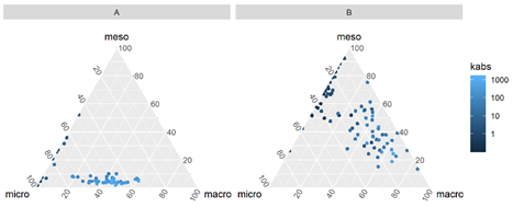
Figure 3.1: Pore-throat class distribution for two sample reservoirs (A and B).
3.1.4 Gaussian Mixture Fit Features
Following the methodology proposed by (Xu and Torres-Verdín 2013), bimodal gaussian mixture distributions, with parameters \(\mu_1\), \(\mu_2\), \(\sigma_1\), \(\sigma_2\), \(\lambda_1\) and \(\lambda_2\), were fitted to each MICP associated pore volume distributions \(p(\log{r})\), using the following approximation.
\[\begin{equation} p(\log{r}) \approx \lambda_1 \frac{1}{\sqrt{2\pi}\sigma_1}\exp{\frac{-(\log{r}-\mu_1)}{2\sigma_1^2}} + \lambda_2 \frac{1}{\sqrt{2\pi}\sigma_2}\exp{\frac{-(\log{r}-\mu_2)}{2\sigma_2^2}} \tag{3.2} \end{equation}\]
\[\begin{equation} \lambda_1 + \lambda_2 = 1 \tag{3.3} \end{equation}\]
The parameters \(\mu_1\), \(\mu_2\), \(\sigma_1\), \(\sigma_2\), \(\lambda_1\) and \(\lambda_2\), provide a compact representation of the MICP associated pore volume distributions \(p(\log{r})\), as exemplified in Figures 3.2 and 3.3.
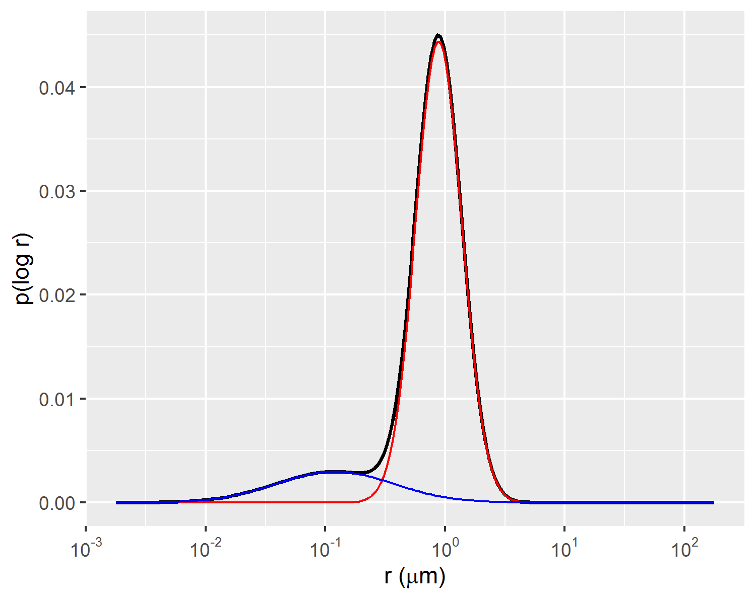
Figure 3.2: Example of bimodal gaussian mixture fit of p(log r) distribution.
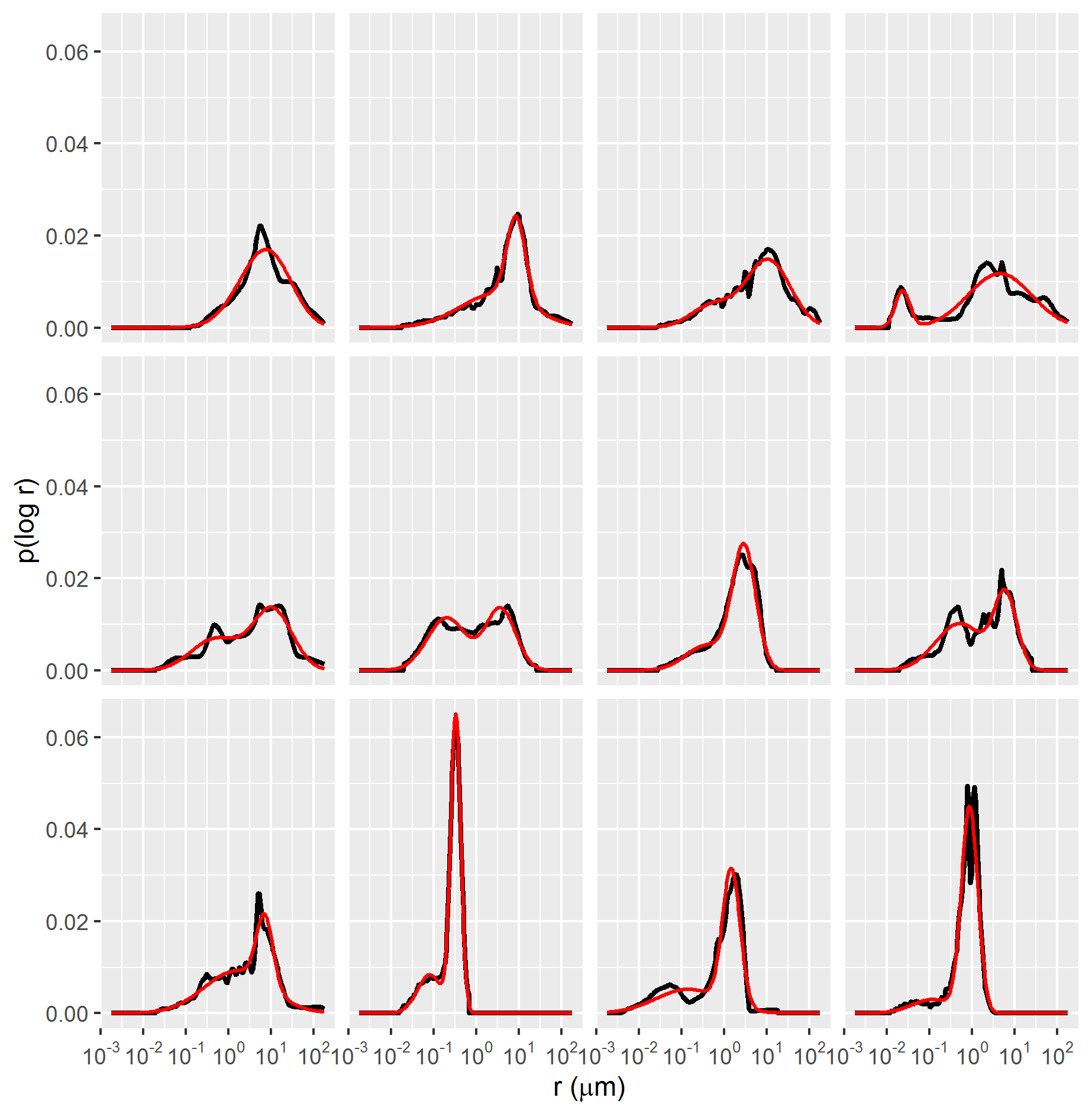
Figure 3.3: Gaussian mixture (red lines) fitted to p(log r) distributions of MICP data samples (black lines).
3.1.5 Dimensionality Reduction Features
Both linear and non-linear dimensionality reduction methods were used to extract features from the dataset of MICP curves. Dimensionality reduction techniques allow for the approximation of the dataset using a lower-dimensional representation, useful for data exploration and visualization and for data compression.
Using as input pore-throat radius quantiles {\(r_{15},r_{20},...,r_{85},r_{90}\)}, the first two principal components PC1 and PC2 were estimated for each of the sample MICP curves using Principal Component Analysis (Hastie, Tibshirani, and Friedman 2009). The first two principal components represented a total of 96.1% of the variance in the dataset. A graphical depiction of the PC1 and PC2 features, colored by absolute permeability can be seen on Figure 3.4.
The first and second principal components were shown to be correlated with absolute permeability \(k_{abs}\) and interquartile range \(iqr\), respectively, as displayed on Figures 3.5 and 3.6.
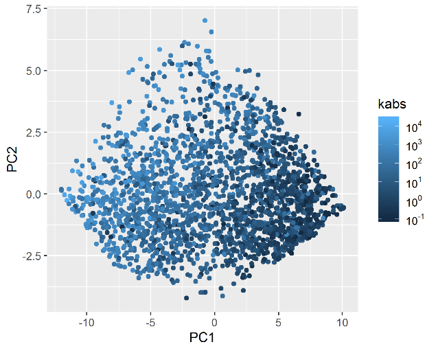
Figure 3.4: First two principal components of each of the datasets MICP samples.

Figure 3.5: Negative correlation between absolute permeability and the first principal component.
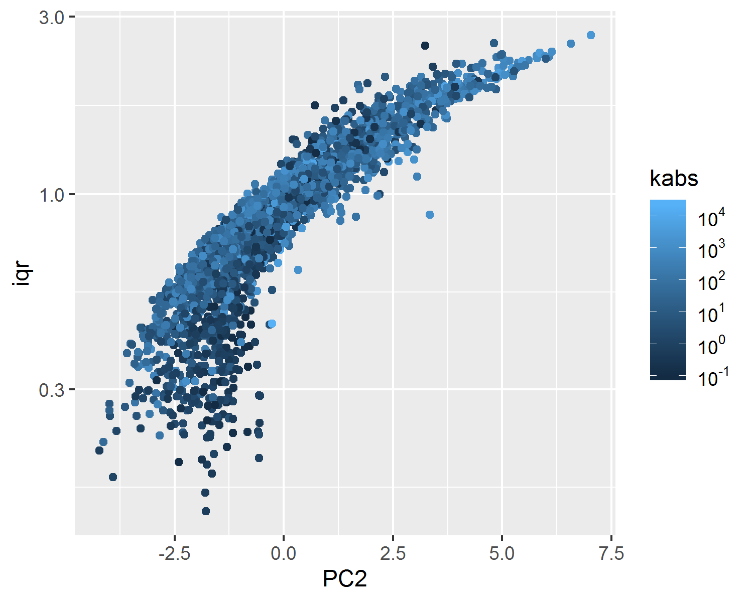
Figure 3.6: Positive correlation between the interquartile-range iqr and the second principal component PC2.
Non-linear dimensionality reduction features were also estimated using Uniform Manifold Approximation and Projection, also known as UMAP (McInnes and Healy 2018), using as input pore-throat radius quantiles {\(r_{15},r_{20},...,r_{85},r_{90}\)}.
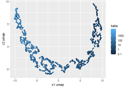
Figure 3.7: MICP curves non-linear decomposition using UMAP.
The Uniform Manifold Approximation and Projection technique constructs a high dimensional graph representation of the data and optimizes a low-dimensional manifold to be as structurally similar to the high dimensional graph as possible (McInnes and Healy 2018). Due to its distance preserving properties, the low-dimensional manifold, represented in Figure 3.7 by variables \(x_1.umap\) and \(x_2.umap\), is useful for visualization and identification of similar MICP curve samples.
In Figure 3.8, this property is exemplified by a sequence of three pairs of plots, showing that samples mapped to the same regions of the UMAP manifold, marked in the red in each of the plot pairs, correspond to distributions \(p(\log{r})\) with similar characteristics.
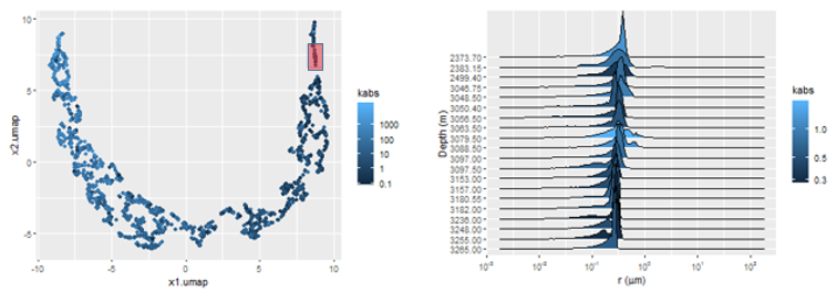
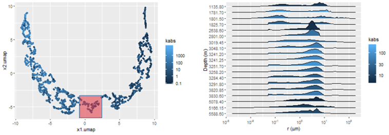
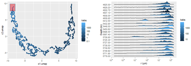
Figure 3.8: Manifold maps (left) showing areas with similar associated pore volume distributions p(log r) (right).
3.2 Absolute Permeability Regression Models
The regression metrics root mean squared error (3.4), median absolute error (3.5) and \(R^2\) (3.6) were evaluated for the trained regression models. Due to the issues regarding the representativeness of the rock fragments with respect to the measured absolute permeability values, discussed on chapter , minimization of the median absolute deviation metric (3.5) was chosen to increase the robustness to outliers of the trained non-linear regression models, described in section . In both linear and non-linear regression methods, the \(R^2\) metric (3.6) was used for further assessment of the trained regression models.
\[\begin{equation} \text{RMSE} = \sqrt{\frac{\sum_{i=1}^n{(\log{\hat{k}_{{abs}_i}}-\log{k_{{abs}_i}})^2}}{n}} \tag{3.4} \end{equation}\]
\[\begin{equation} \text{MAE} = \frac{\sum_{i=1}^n{|\log{\hat{k}_{{abs}_i}}-\log{k_{{abs}_i}}}|}{n} \tag{3.5} \end{equation}\]
\[\begin{equation} R^2 = 1-\frac{\sum_{i=1}^n{(\log{\hat{k}_{{abs}_i}}-\log{k_{{abs}_i}})^2}}{\sum_{i=1}^n{(\log{k_{{abs}_i}}-\overline{\log{k_{{abs}_i}}})^2}} \tag{3.6} \end{equation}\]
3.2.1 Linear Regression Models
The linear features, described in section , were used to fit linear regression logarithmic absolute permeability \(\log{k_{abs}}\) models.
Among the fitted linear regression models, the Winland and Swanson models obtained the lowest root mean squared error and highest coefficient of determination metrics.
Figure 3.9 shows a graphical representation of the fitted models, where a significant number of outlier logarithmic absolute permeability estimates \(\log{\hat{k}_{abs}}\) , with more than one order of magnitude errors, can be seen. The presence of this large number of outliers can be explained by the limited rock fragment representativeness of the core sample pore volume for heterogeneous reservoirs, described in chapter .
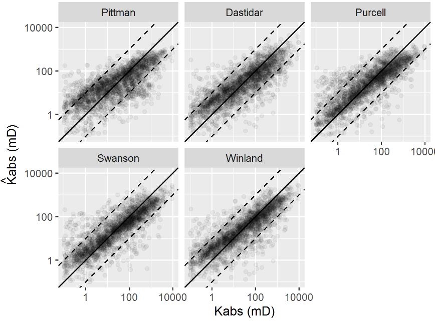
Figure 3.9: Visual evaluation of the predicted and observed absolute permeability models using linear features.
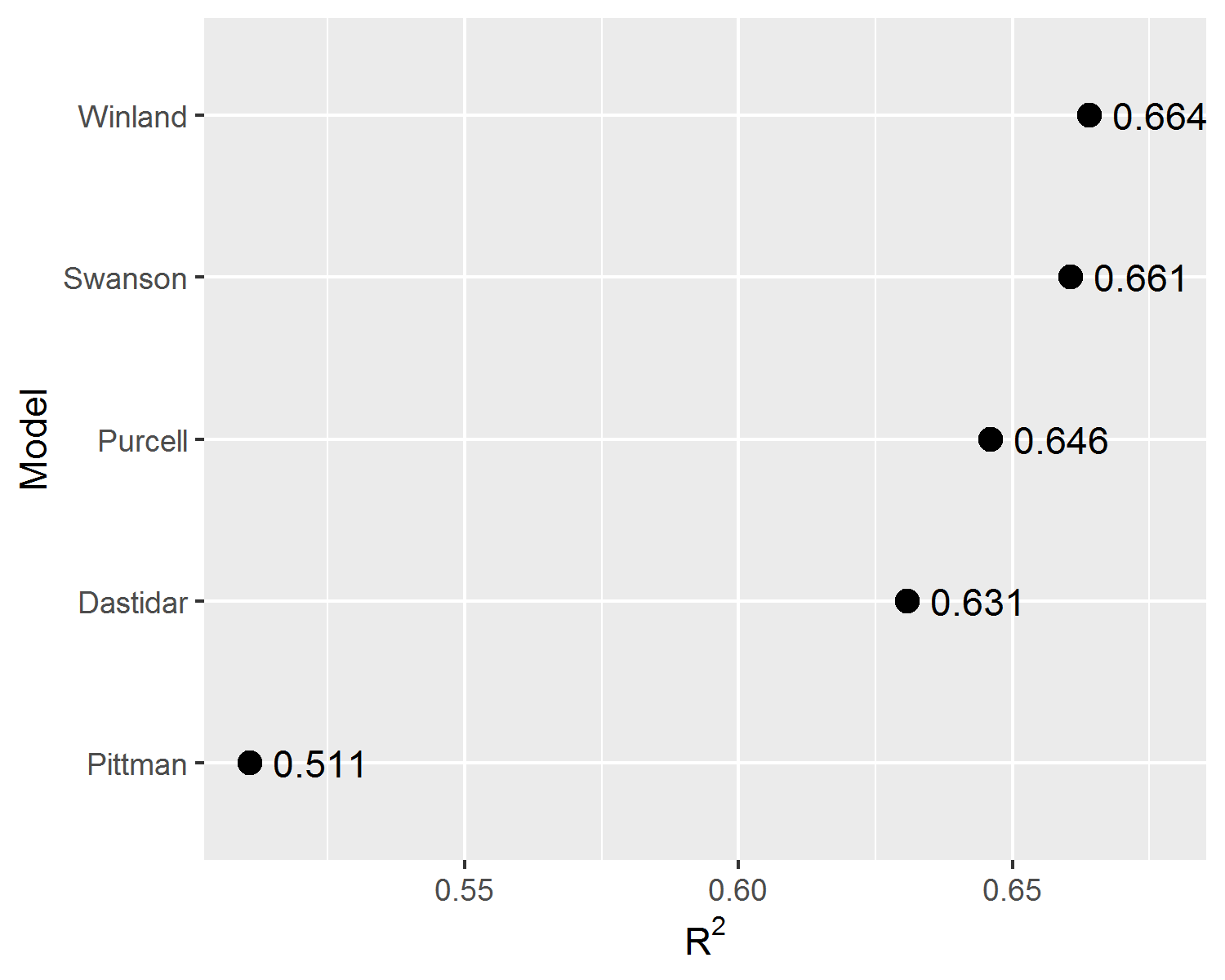
Figure 3.10: Comparison of the \(R^2\) metric for the fitted linear regression models.
3.2.2 Black-Box Machine Learning Models
Using the features described in section , six additional non-linear regression models were fit to the dataset using machine learning models. The 2324 MICP curves were split between training and test data, with a eighty to twenty percent ratio. Using the training set, each algorithm went through a hyper-parameter tuning procedure, using ten times repeated five-fold cross-validation error estimation, on a grid of selected hyper-parameters.
Two \(knn\) nearest neighbors models (P. Murphy 2012), were fit to the training set, one using features extracted using PCA (Hastie, Tibshirani, and Friedman 2009) and the other features extracted using UMAP non-linear dimensionality reduction (McInnes and Healy 2018).
A simple linear regression model was fit using the features extracted from the bi-modal gaussian mixture model proposed by (Xu and Torres-Verdín 2013), described in section .
A support vector regression (SVR) model, a random forest model and a gradient boosted trees model (Hastie, Tibshirani, and Friedman 2009) were fit to an expanded feature set, consisting of the features proposed by Swanson, Winland, Purcell, the sample porosity \(\phi\), the micropores and mesopores ternary class distributions, the UMAP features and the bi-modal gaussian mixtures distribution features. A pre-processing standardizing step was applied to each feature. The gradient boosted trees model was fitted using the implementation provided by the XGBoost library (Chen and Guestrin 2016).
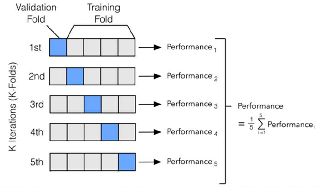
Figure 3.11: Five-fold cross-validation procedure.
Table 3.2 and Figure 3.12 show median values of repeated five-fold cross-validated MAE, \(R^2\) and RMSE metrics for each of the trained regression models. The regression models with the lowest median absolute error were the SVR, randomForest and gradient boosted trees XGB models. Through the use of a radial basis function kernel and an optimization procedure that minimizes hinge loss (Hastie, Tibshirani, and Friedman 2009), the SVR algorithm provides outlier robust predictions. The random forest and gradient boosted trees algorithms use randomized selection of features and data subsets, bagging and boosting techniques, respectively, to reduce prediction errors of ensembles of simpler decision tree models (Chen and Guestrin 2016).
| Regression Model | MAE | \(R^2\) | RMSE |
|---|---|---|---|
| SVR | 0.412 | 0.722 | 0.596 |
| randomForest | 0.437 | 0.712 | 0.604 |
| XGB | 0.439 | 0.711 | 0.605 |
| Swanson | 0.471 | 0.681 | 0.639 |
| GaussianMixture | 0.477 | 0.675 | 0.641 |
| Winland | 0.481 | 0.674 | 0.643 |
| Purcell | 0.487 | 0.661 | 0.654 |
| Dastidar | 0.520 | 0.642 | 0.673 |
| knnUMAP | 0.565 | 0.562 | 0.744 |
| knnPCA | 0.581 | 0.547 | 0.753 |
| Pittman | 0.613 | 0.523 | 0.775 |
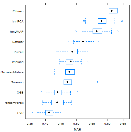
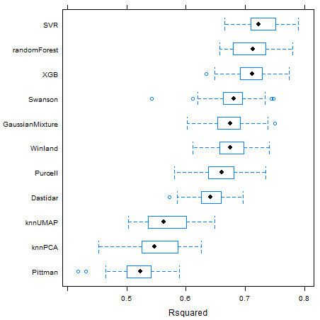
Figure 3.12: Boxplots for repeated five-fold cross-validated MAE, \(R^2\) and RMSE metric results for each model.
Non-linear machine learning models presented consistently lower prediction errors, as can be seen on Figure 3.12. On Figure 3.13, a visual comparison between linear and non-linear machine learning models of the predicted versus measured data for the test dataset is shown. Although the non-linear machine-learning models did obtain better MAE, \(R^2\) and RMSE metrics results, a significant number of outliers are still present, probably related to the issue of limited rock fragment representativeness of highly heterogeneous reservoirs described in chapter .
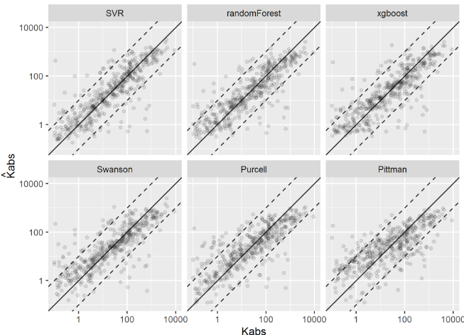
Figure 3.13: Visual evaluation of the estimated absolute permeability models using Machine Learning and linear models.
References
Al Khalifah, H., P. W. J. Glover, and P. Lorinczi. 2020. “Permeability prediction and diagenesis in tight carbonates using machine learning techniques.” Marine and Petroleum Geology 112 (May 2019): 104096. https://doi.org/10.1016/j.marpetgeo.2019.104096.
Chen, Tianqi, and Carlos Guestrin. 2016. “XGBoost: A scalable tree boosting system.” Proceedings of the ACM SIGKDD International Conference on Knowledge Discovery and Data Mining 13-17-Augu: 785–94. https://doi.org/10.1145/2939672.2939785.
Hastie, Trevor, Robert Tibshirani, and Jerome Friedman. 2009. The Elements of Statistical Learning: Data Mining, Inference, and Prediction.
Kolodzie, Stanley. 1980. “Analysis of Pore Throat Size and Use of the Waxman-Smits Equation to Determine Ooip in Spindle Field, Colorado.” In SPE Annual Technical Conference and Exhibition, 10. Dallas, Texas: Society of Petroleum Engineers. https://doi.org/10.2118/9382-MS.
McInnes, L., and J. Healy. 2018. “UMAP: Uniform Manifold Approximation and Projection for Dimension Reduction.”
Nooruddin, Hasan A., Fatai Anifowose, and Abdulazeez Abdulraheem. 2013. “Applying Artificial Intelligence Techniques to Develop Permeability Predictive Models using Mercury Injection Capillary-Pressure Data.” SPE Saudi Arabia Section Technical Symposium and Exhibition, 1–16. https://doi.org/10.2118/168109-MS.
Pittman, E. D. 1992. “Relationship of porosity and permeability to various parameters derived from mercury injection-capillary pressure curves for sandstone.” https://doi.org/10.1017/CBO9781107415324.004.
P. Murphy, Kevin. 2012. Machine Learning: A Probabilistic Perspective. https://doi.org/10.1007/SpringerReference_35834.
Purcell, W. R. 1949. “Capillary Pressures - Their Measurement Using Mercury and the Calculation of Permeability Therefrom.” Journal of Petroleum Technology 1 (02): 39–48. https://doi.org/10.2118/949039-G.
Swanson, B. F. 1981. “A Simple Correlation Between Permeabilities and Mercury Capillary Pressures.” Journal of Petroleum Technology 33 (12): 2498–2504. https://doi.org/10.2118/8234-PA.
Xu, C., and C. Torres-Verdín. 2013. “Pore System Characterization and Petrophysical Classification Using a Bimodal Gaussian Density Function.” Math Geosci.