Chapter 4 Hierarchical Multi-Task Linear Regression

Linear regression methods are widely used in petrophysical characterization. Compared to non-linear machine learning models, they have as advantages simplicity, interpretability and their inherent linear behavior on extrapolated predictions. For the estimation of special core analysis properties, which are costly to acquire and thus usually scarce, simple models with a low number of parameters and that can deliver interpretable probabilistic inferences are highly desirable. In this work, two different linear regression techniques are evaluated on special core analysis datasets.

On a dataset containing 135 capillary pressure curves estimated from centrifuge experiments, a multi-task linear regression model is fit and evaluated, and some of its properties are analyzed.

On another dataset, containing 226 unsteady-state water-oil relative permeability curves, partially pooled hierarchical linear regression models are evaluated and compared to simple linear regression models.

4.1 Multi-Task Linear Regression

Using the parameterization (4.1), proposed by (Albuquerque et al. 2018), a dataset containing parameters \(S_{wi}\), \(P_e\), \(\alpha\) and \(\beta\) fitted to each of the available 135 centrifuge capillary pressure curves, was assembled.

\[\begin{equation} S_w(P_c, S_{wi}, P_e, \alpha, \beta) = \frac{1+\alpha S_{wi}(P_c - P_e)^\beta}{1+\alpha (P_c - P_e)^\beta} \tag{4.1} \end{equation}\]

To each of these samples, features extracted from MICP curves obtained on corresponding rock fragments were associated in a dataset containing {\(S_{wi}\), \(P_e\), \(\alpha\), \(\beta\), \(k_{abs}\), \(r_{35}\), \(iqr\)} values for each MICP and centrifuge capillary pressure curve pair. Significant correlations between corresponding centrifuge capillary pressure curves \(\alpha\), \(S_{wi}\) and MICP median pore throat radius \(r_{median}\) parameters can be visualized in Figure 4.2.

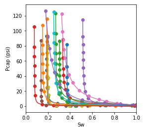
Figure 4.1: Sample of the experimental capillary pressure curve dataset (points) and fitted capillary pressure model (lines).

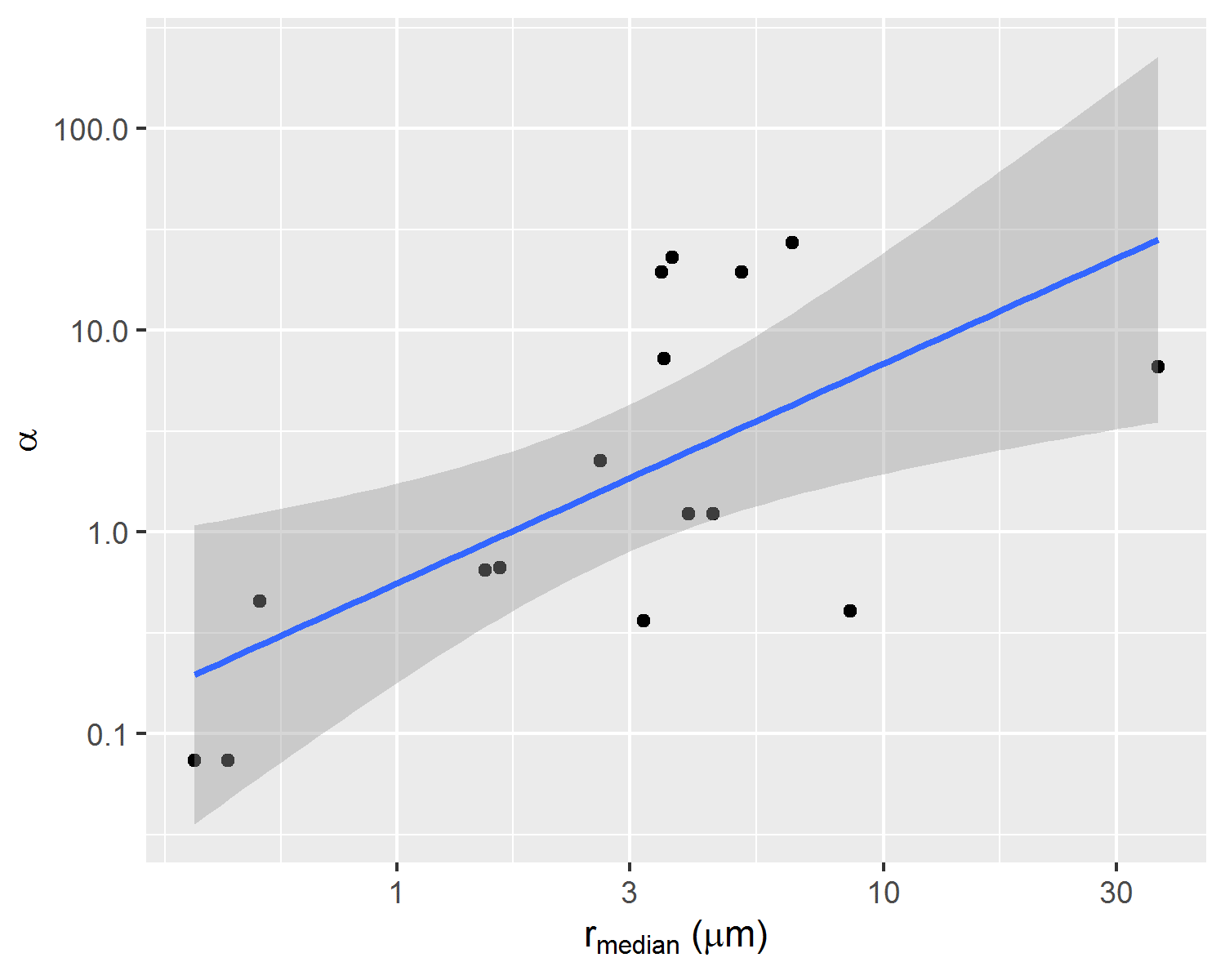
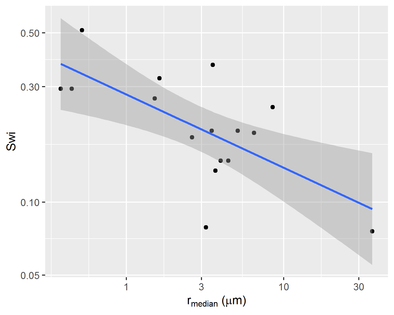
Figure 4.2: Correlations between parameters alpha, Swi and median pore throat radius of correspondent rock fragment p(log r) distribution.

Given \(x\) a vector of input parameters {\(k_{abs}\), \(r_{35}\), \(iqr\)} and y a vector of output parameters {\(S_{wi}\), \(\alpha\), \(\beta\), \(P_e\)}, and considering a multivariate gaussian distribution described by equation (4.2), the conditional distribution of the output parameters given known input parameters \(p(y|x)\) may be described by equations (4.3)(4.4)(4.5). Estimating mean and covariance matrix statistics of the multivariate gaussian distribution (4.2) on the assembled dataset, using maximum likelihood methods (DeGroot and Schervish 2012), inference and uncertainty evaluation may be performed on desired new input \(x\) values.

\[\begin{equation} \begin{pmatrix} x \\ y \end{pmatrix} \sim \mathcal{N}\left(\begin{pmatrix} \mu_x \\ \mu_y \end{pmatrix},\begin{pmatrix} \Sigma_{xx} & \Sigma_{xy} \\ \Sigma_{yy} & \Sigma_{xy} \end{pmatrix}\right) \tag{4.2} \end{equation}\]

\[\begin{equation} p(y|x) \sim \mathcal{N}(\mu_{y|x}, \Sigma_{y|x}) \tag{4.3} \end{equation}\]

\[\begin{equation} \mu_{y|x} = \mu_y + (\Sigma_{xx}^{-1}\Sigma_{yx})^t(x-\mu_x) \tag{4.4} \end{equation}\]

\[\begin{equation} \Sigma_{y|x} = \Sigma_{yy} - \Sigma_{xy}^{t}\Sigma_{xx}^{-1}\Sigma_{yx} \tag{4.5} \end{equation}\]

Given new \(x=\{k_{abs}, r_{35}, iqr\}\) values, the expected capillary pressure curve parameters \(E[y|x]\) may be obtained by the conditional mean \(\mu_{y|x}\). Uncertainty evaluation of this prediction may be executed using samples of the conditional distribution \(p(y|x)\). Figure 4.3 displays examples of experimental capillary pressure curves and predictions of these curves using as input associated \(\{k_{abs}, r_{35}, iqr\}\) values. Samples from the conditional distribution \(p(y|x)\) are shown as grey lines and illustrate prediction uncertainty.

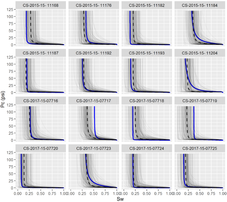
Figure 4.3: Visual comparison of experimental capillary pressure curves (blue lines), samples from the conditional distribution (grey lines) and average predicted curves (dashed black lines).

On Figure 4.4, a comparison between experimental and predicted capillary pressure curve parameters is shown. Due to inherent noise associated with heterogeneous reservoir rocks and, as also observed in Figure 4.3, there is significant dispersion of experimental and predicted parameters values. Both in Figures 4.4 and 4.5, it is possible to visualize that capillary curve parameter predictions follow linear tendencies with absolute permeability. This property of linear model predictions is desirable, as it follows the expected physical behavior of reservoir rocks.

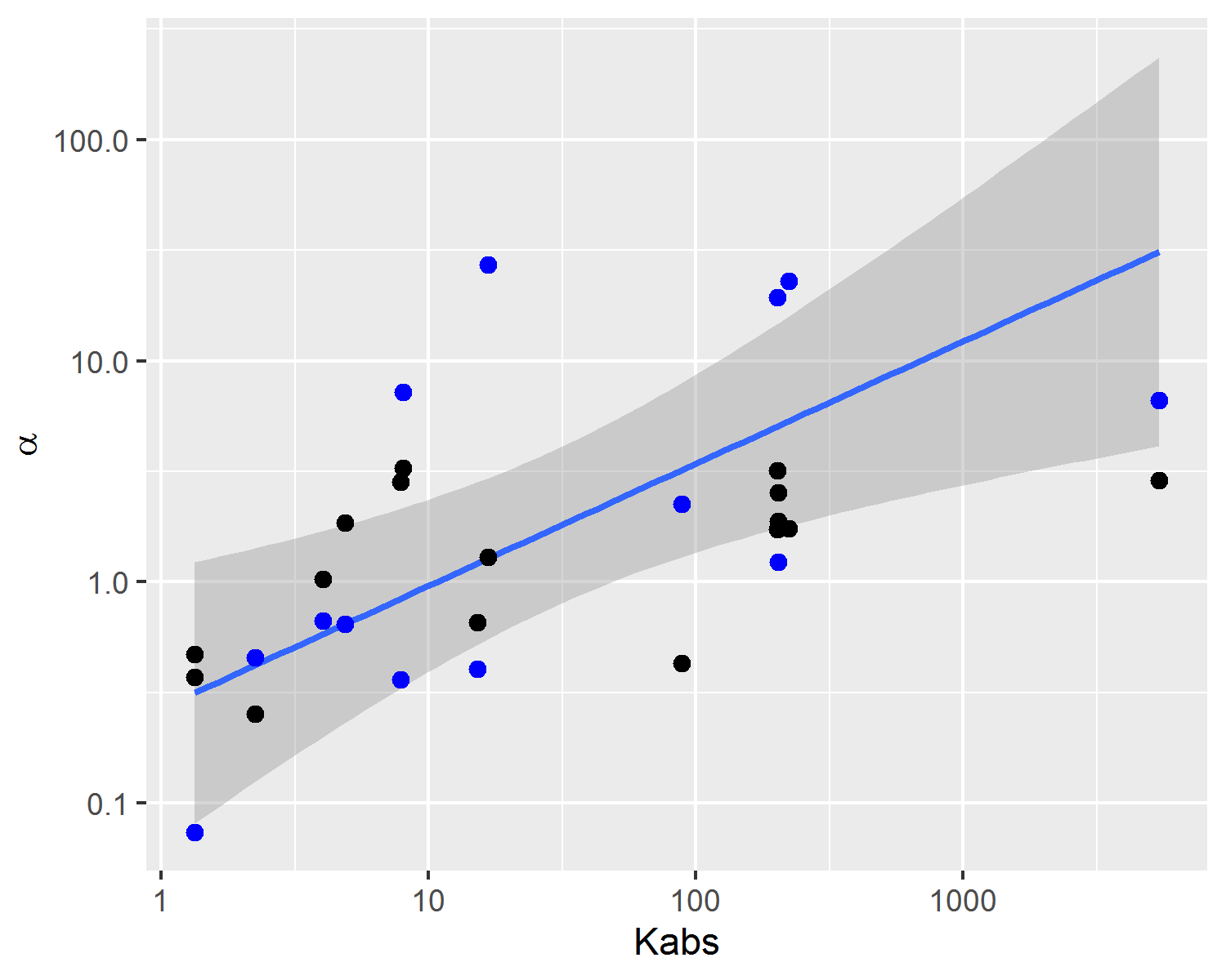
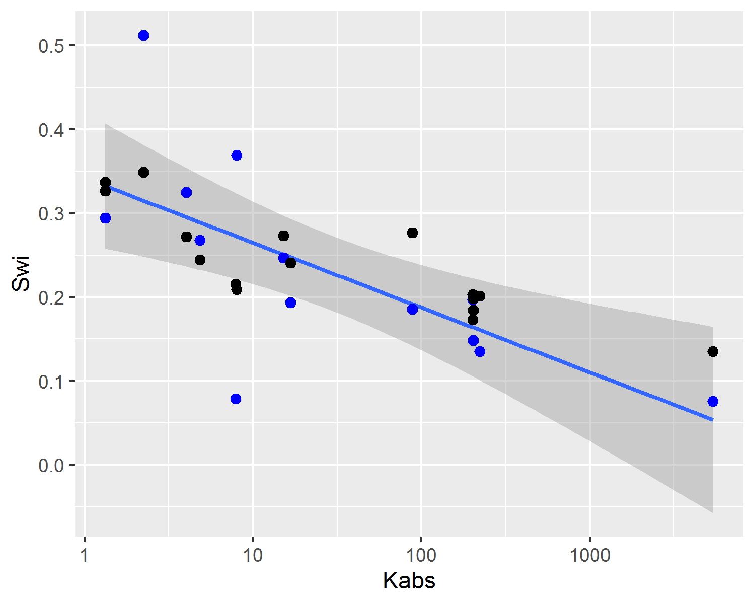
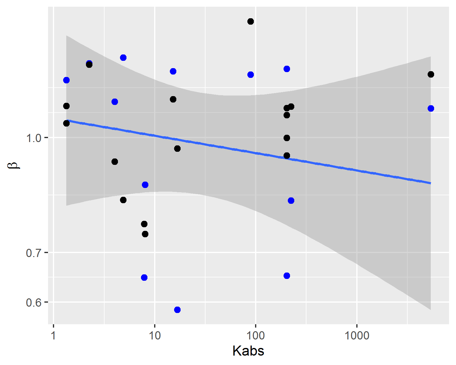
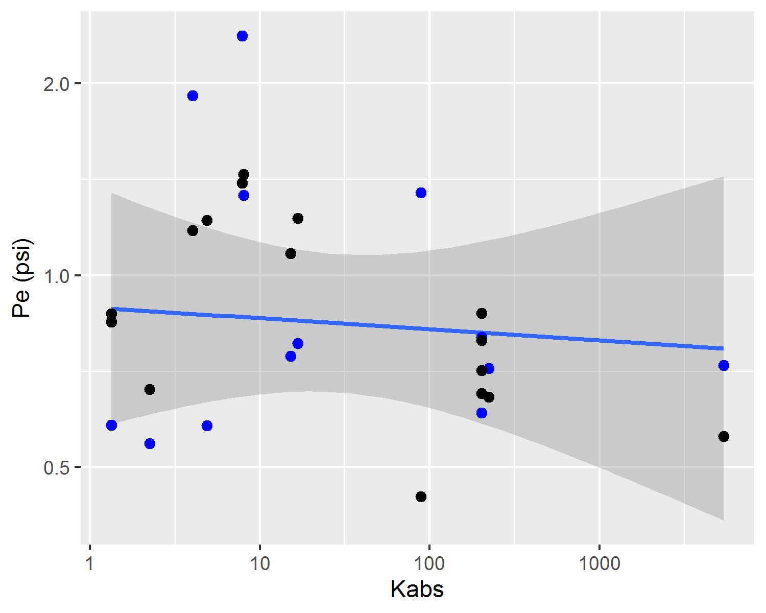
Figure 4.4: Experimental capillary pressure curve parameters (blue dots and line tendency) and predicted parameters estimated using the posterior mean (black dots).

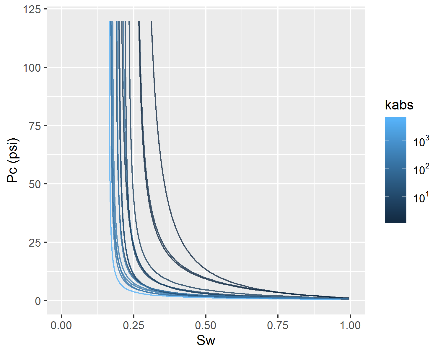
Figure 4.5: Behaviour of predicted capillary pressure curves with absolute permeability.

4.2 Hierarchical Linear Regression

In a reservoir model, the prediction of petrophysical properties on simulation cells distant from wells with available sampled cores is commonly performed using linear regression methods (Peters 2012). To account for sampling bias, special core analysis properties such as relative permeability and capillary pressure are commonly scaled according to reservoir wide available information, such as absolute permeability, porosity and geological facies models. For relative permeability, this procedure is commonly performed using simple linear regression (Gelman et al. 2014) of relative permeability parameters as a function of absolute permeability.

On this work, simple linear and hierarchical linear regression models were evaluated in a dataset containing 226 unsteady-state water-oil relative permeability curves from several Brazilian reservoirs. Parameters for each of the 226 curves were fitted using maximum likelihood estimation (Migon, Gamerman, and Louzada 2015) and the LET parameterization (4.6)(4.7)(4.8) proposed in (Lomeland, Ebeltoft, and Thomas 2005).

\[\begin{equation} S_{wD} = \frac{S_w - S_{wi}}{1 - S_{wi} - S_{or}} \tag{4.6} \end{equation}\]

\[\begin{equation} k_{ro}(S_w) = k_{ro@S_{wi}}\frac{(1-S_{wD})^{L_o}}{(1-S_{wD})^{L_o} + E_o(S_{wD})^{T_o}} \tag{4.7} \end{equation}\]

\[\begin{equation} k_{rw}(S_w) = k_{rw@S_{or}}\frac{(S_{wD})^{L_w}}{(S_{wD})^{L_w} + E_w(1-S_{wD})^{T_w}} \tag{4.8} \end{equation}\]

Categorical variables, such as field, reservoir or geological facies, may be used to group petrophysical models. A model that does not distinguish between groups, using constant intercept and slope parameters for all categories according to equation (4.9), may be referred to as a non-pooled model (Gelman et al. 2014). Figure 4.6 displays a simple linear non-pooled regression model of irreducible water saturation \(S_{wi}\) as the predicted \(y\) variable and the logarithm of absolute permeability \(\log{k_{abs}}\) as the observed \(x\) variable. On equation (4.9), \(n\) represents the total number of data samples, indexed by the letter \(i\), and \(\alpha\), \(\beta\) and \(\sigma_y^2\) represent the intercept, slope and variance linear model parameters.

\[\begin{equation} y_i \sim \mathcal{N}(\alpha + \beta x, \sigma_y^2),\quad \text{for}\; i=1,...,n \tag{4.9} \end{equation}\]

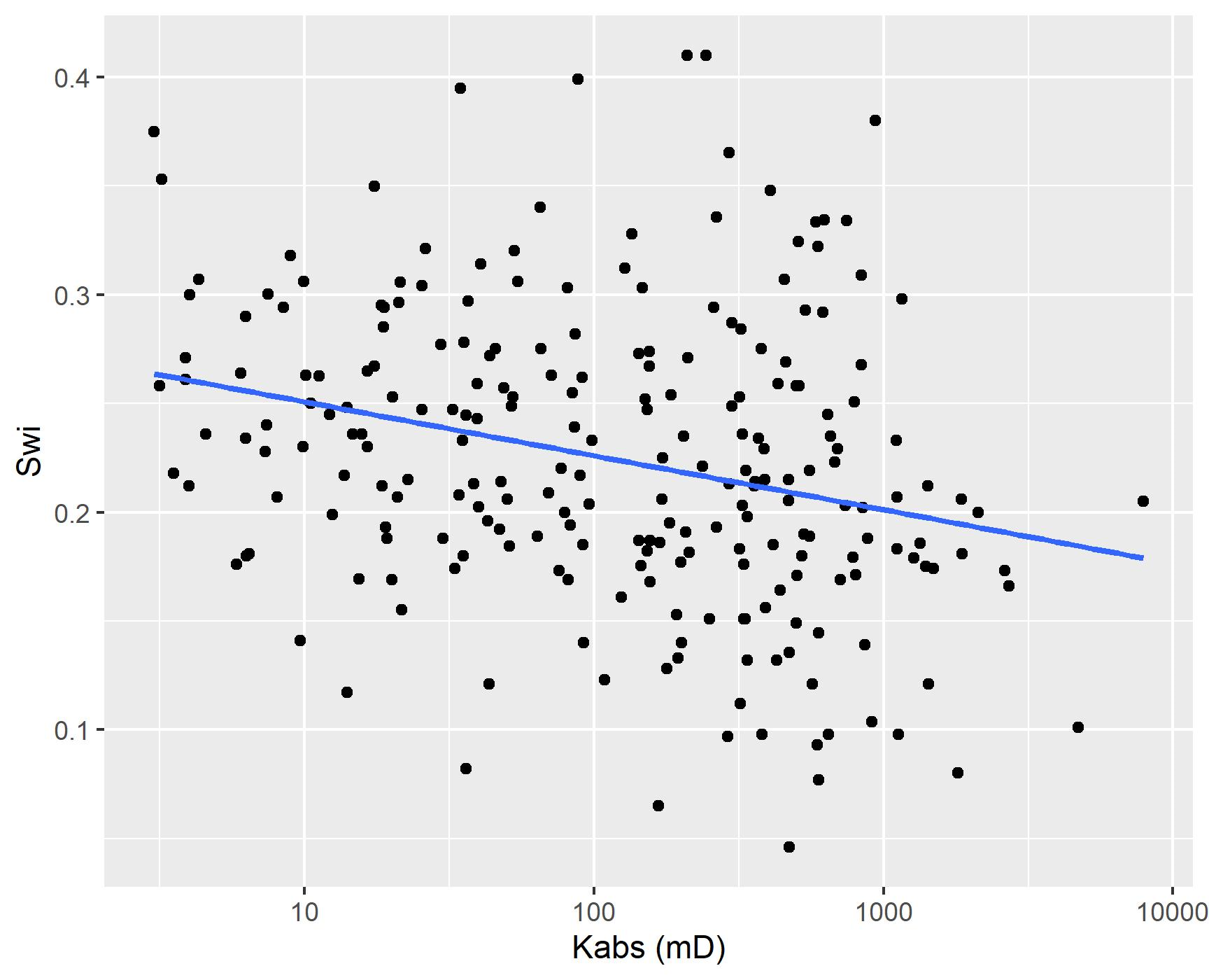
Figure 4.6: Non-pooled simple linear regression.

Usually, though, separate linear regression models are fitted to each category of interest, in models that may be referred to as completely pooled. For each category \(j\), independent \(\alpha_j\), \(\beta_j\) and \(\sigma_{y^j}^2\) parameters are estimated, as described in equation (4.10).

\[\begin{equation} y_i^j \sim \mathcal{N}(\alpha_j + \beta_j x_i^j, \sigma_{y^j}^2),\quad \text{for}\; i=1,...,n; \quad \text{for} \; i=1,...,J \tag{4.10} \end{equation}\]

Figure 4.7 displays a simple linear completely pooled regression model of irreducible water saturation \(S_{wi}\) and the logarithm of absolute permeability \(\log{k_{abs}}\), grouped by reservoir. In completely pooled regression models, each linear regression model is independent of each other, with varying degrees of uncertainty on each model parameters \(\alpha_j\), \(\beta_j\) and \(\sigma_{y^j}^2\). Categories with larger number of samples and smaller heterogeneities, usually display smaller uncertainties on model parameters.

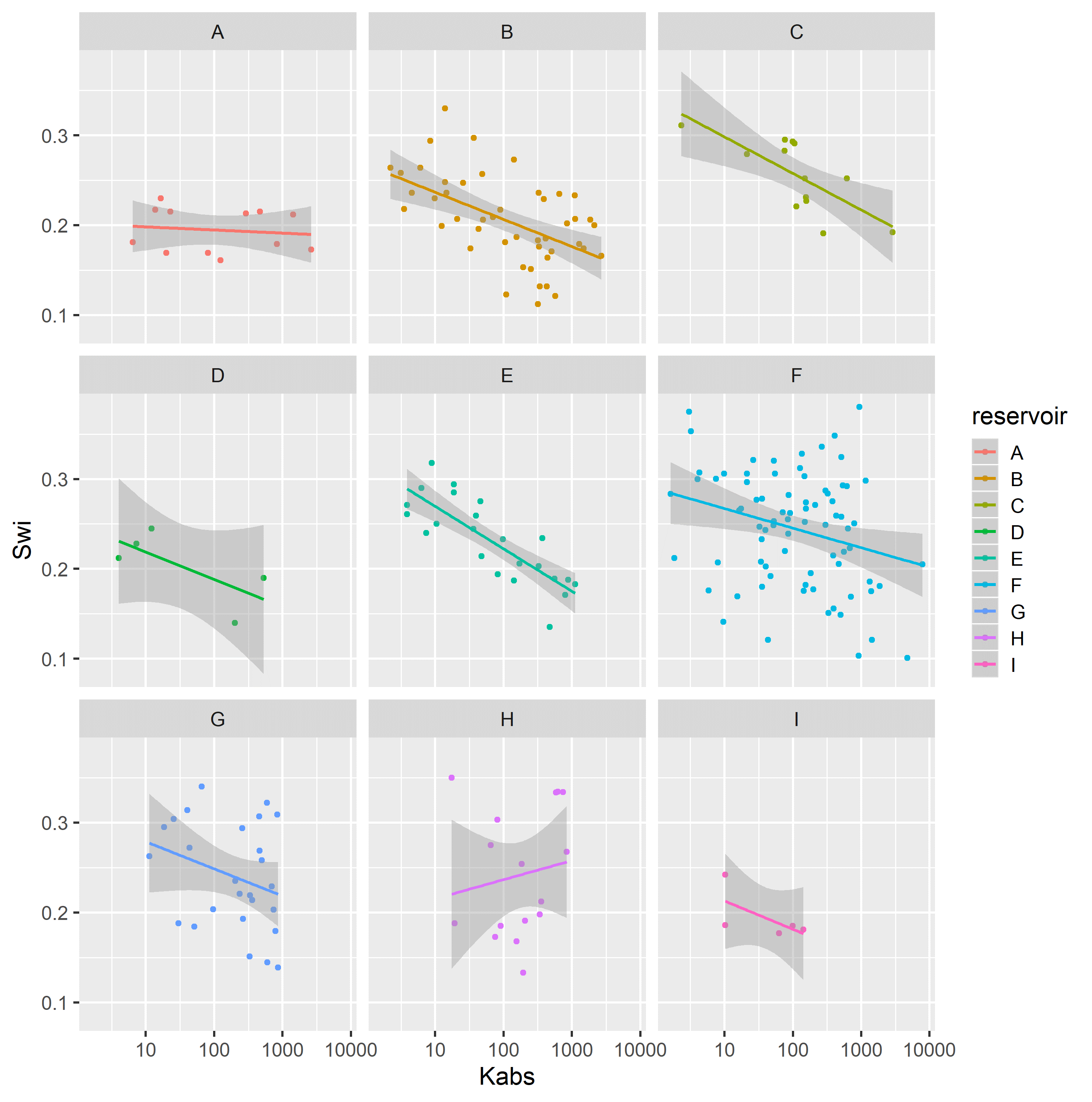
Figure 4.7: Completely pooled simple linear regression models, grouped by reservoir.

Hierarchical or partially pooled linear regression models introduce information sharing and coupling between model parameters of different categories, modeling intercept and/or slope parameters as sampled from a latent parent distribution.

Varying intercept models, assume that the intercept of each category \(\alpha_j\) is sampled from a common latent gaussian distribution (4.12). This information sharing, has a regularizing effect of shrinking the partially pooled parameters towards a common mean \(\mu_\alpha\).

\[\begin{equation} y_i^j \sim \mathcal{N}(\alpha_j + \beta_j x_i^j, \sigma_{y^j}^2),\quad \text{for}\; i=1,...,n; \quad \text{for} \; j=1,...,J \tag{4.11} \end{equation}\]

\[\begin{equation} \alpha_j \sim \mathcal{N}(\mu_\alpha, \sigma_\alpha^2), \quad \text{for} \; j=1,...,J \tag{4.12} \end{equation}\]

Varying slope models, assume that the slope of each category \(\beta_j\) is sampled from a common latent gaussian distribution (4.14), with the same regularizing effect of shrinking the partially pooled parameters towards a common mean \(\mu_\beta\).

\[\begin{equation} y_i^j \sim \mathcal{N}(\alpha_j + \beta_j x_i^j, \sigma_{y^j}^2),\quad \text{for}\; i=1,...,n; \quad \text{for} \; j=1,...,J \tag{4.13} \end{equation}\]

\[\begin{equation} \beta_j \sim \mathcal{N}(\mu_\beta, \sigma_\beta^2), \quad \text{for} \; j=1,...,J \tag{4.14} \end{equation}\]

Varying intercept and slope models, assume that both the intercept and slope of each category \(\alpha_j\) and \(\beta_j\) are sampled from a common latent multivariate gaussian distribution (4.16).

\[\begin{equation} y_i^j \sim \mathcal{N}(\alpha_j + \beta_j x_i^j, \sigma_{y^j}^2),\quad \text{for}\; i=1,...,n; \quad \text{for} \; j=1,...,J \tag{4.15} \end{equation}\]

\[\begin{equation} \begin{pmatrix} \alpha_j \\ \beta_j \end{pmatrix} \sim \mathcal{N}\left(\begin{pmatrix} \mu_\alpha \\ \mu_\beta \end{pmatrix},\begin{pmatrix} \sigma_\alpha^2 & \rho \sigma_\alpha \sigma_\beta \\ \rho \sigma_\alpha \sigma_\beta & \sigma_\beta^2 \end{pmatrix}\right),\quad \text \quad \text{for} \; j=1,...,J \tag{4.16} \end{equation}\]

For the dataset of 226 unsteady-state water-oil relative permeability curve LET parameters, hierarchical varying slope models of relative permeability endpoint parameters \(S_{wi}\), \(S_{or}\), \(k_{ro}@S_{wi}\) and \(k_{rw}@S_{or}\), and logarithm of absolute permeability \(\log{k_{abs}}\) were fit and compared to completely pooled simple linear regression models, grouped by reservoir.

Both hierarchical and simple linear regression model parameters were inferred using bayesian Hamiltonian Markov-Chain Monte-Carlo (Hoffman and Gelman 2014) and the software Stan (Carpenter et al. 2017). Default weakly informative model parameter priors were utilized, following the recommendations of (Gelman et al. 2008).

Comparison between hierarchical and simple linear regression models were performed using the root mean squared error RMSE, the Watanabe-Akaike Information Criteria (WAIC), the leave-one-out information criteria (LOOIC), and the bayesian R-squared \(R^2\) and adjusted R-squared \(R_{adj}^2\) metrics (Gelman et al. 2019)(Vehtari, Gelman, and Gabry 2017). The WAIC and LOOIC information criteria provide a trade-off between goodness-of-fit and model complexity, with lower WAIC and LOOIC values corresponding to lower cross-validation errors.

Hierarchical varying slope and simple linear regression models of irreducible water saturation \(S_{wi}\) and logarithm of absolute permeability \(\log{k_{abs}}\) were evaluated on the assembled dataset.

Table 4.1 displays the obtained regression metrics for each fitted model. Hierarchical linear regression achieved slightly better WAIC, LOOIC and \(R_{adj}^2\) metrics.

Table 4.1: \(S_{wi}\) linear regression model metrics.

Regression Model	RMSE	WAIC	LOOIC	\(R^2\)	\(R_{adj}^2\)
Simple Linear Regression	0.05	-681.48	-680.96	0.20	0.16
Hierarchical Linear Regression	0.05	-684.89	-684.66	0.24	0.17

Figure 4.8 displays simple and hierarchical linear regression \(S_{wi}\) vs \(\log{k_{abs}}\) models, grouped by reservoir. Black dots represent observed samples, light blue lines represent samples from the posterior distribution of intercept and slope parameters, and dark blue lines represent mean intercept and slope parameters, for each reservoir.

Completely pooled, simple linear regression models display larger between-groups slope variations and uncertainty, as shown in Figure 4.9. Reservoirs with large number of samples, such as reservoir F, display only small changes between hierarchical and simple linear regression model posterior distributions. A stronger regularizing effect is displayed in reservoir H, which contains a small number of samples. Overall behavior consistency of \(S_{wi}\) with respect to \(\log{k_{abs}}\) is increased in the hierarchical partially pooled linear model, as slopes are regressed towards a common mean. As information is shared between different reservoirs, posterior uncertainties are noticeably reduced in the hierarchical linear model.

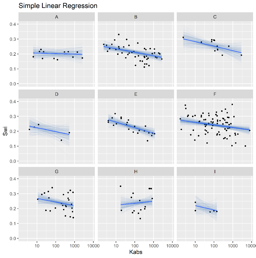
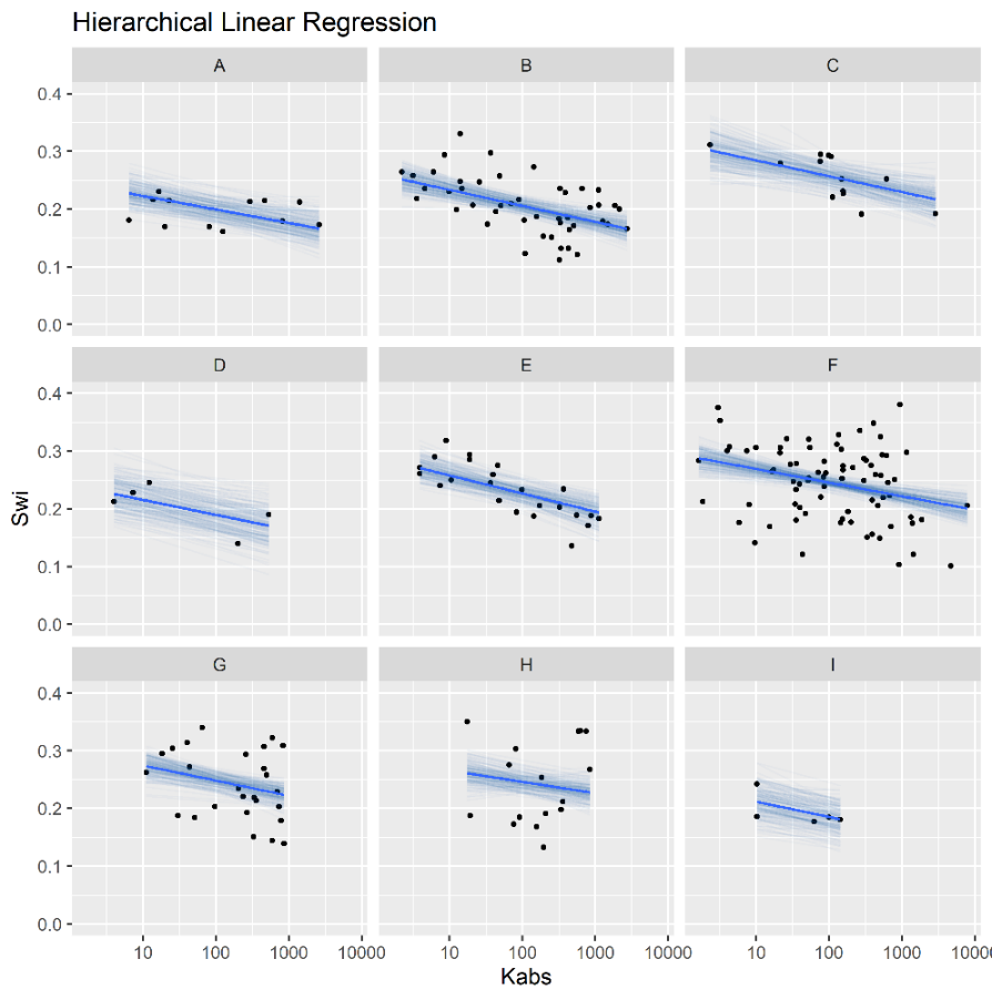
Figure 4.8: Simple (top) and Hierarchical (bottom) linear regression models of Swi vs log(kabs), grouped by reservoir.

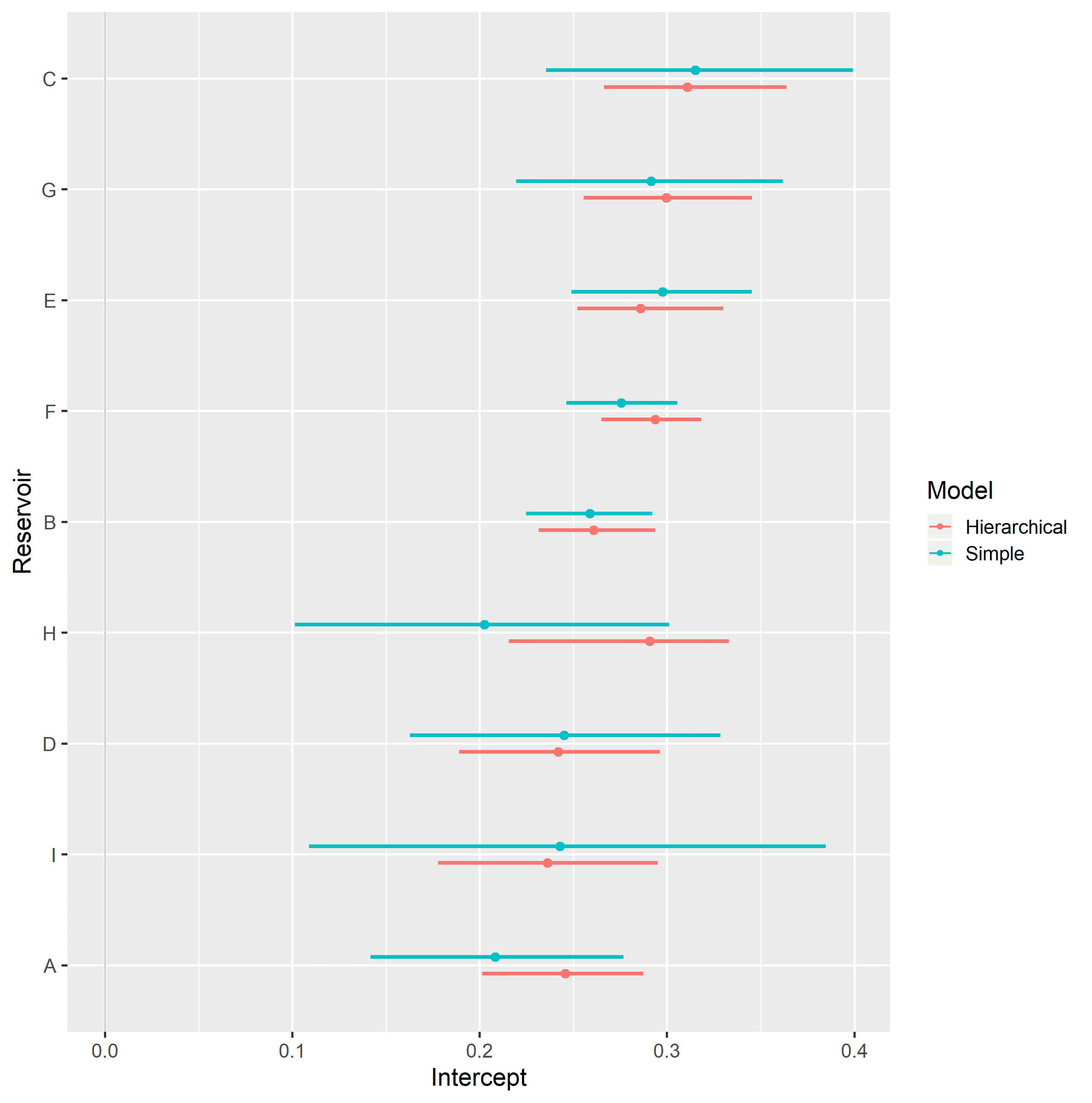
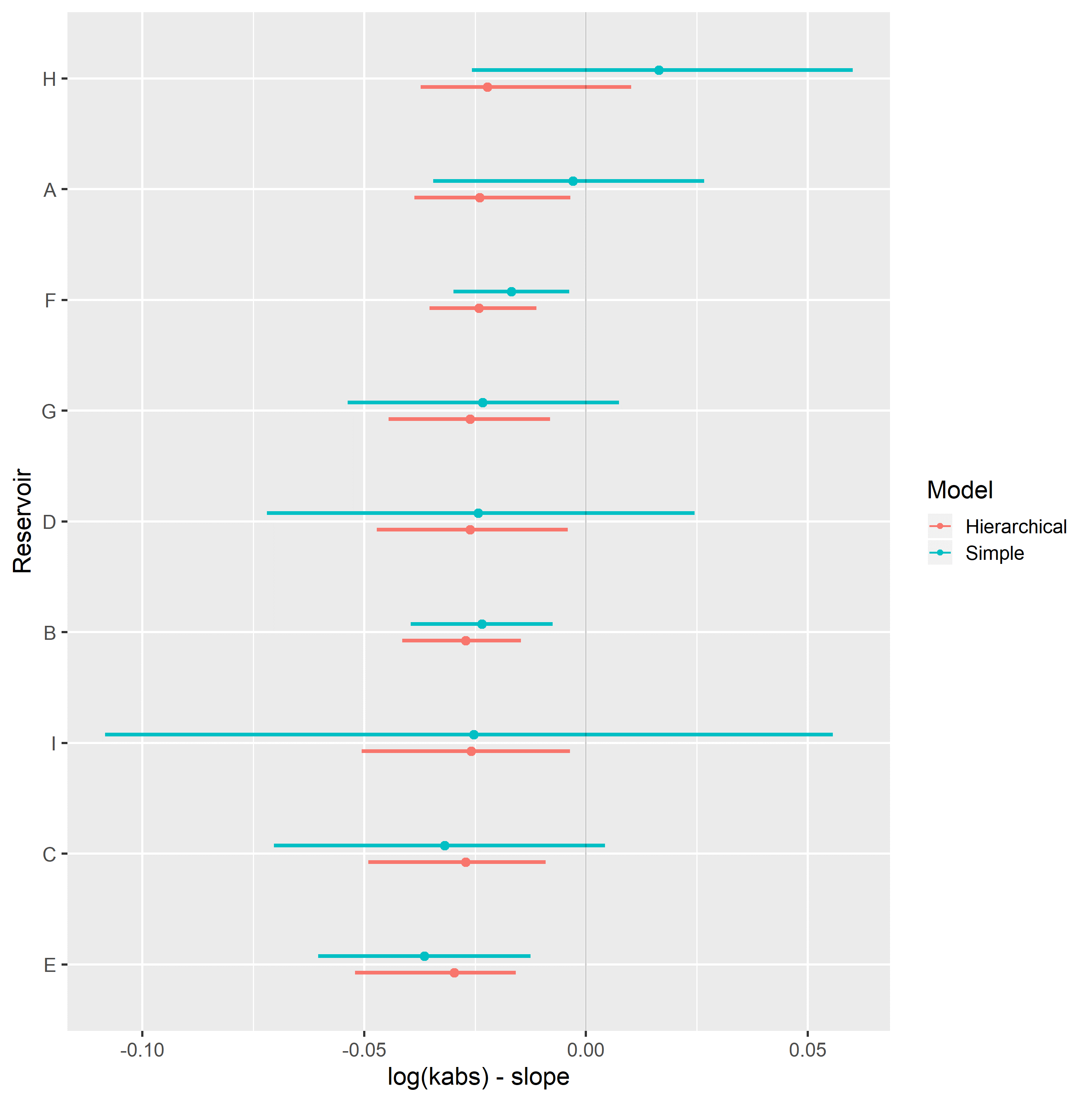
Figure 4.9: Intercept (top) and slope (bottom), simple and hierarchical linear regression Swi vs log(kabs) model parameters, grouped by reservoir.

Hierarchical varying slope and simple linear regression models of residual oil saturation \(S_{or}\) and logarithm of absolute permeability \(\log{k_{abs}}\) were evaluated on the assembled dataset.

Table 4.2 displays the obtained regression metrics for each fitted model. Both models achieved similar WAIC, LOOIC and \(R_{adj}^2\) metrics.

Table 4.2: \(S_{or}\) linear regression model metrics.

Regression Model	RMSE	WAIC	LOOIC	\(R^2\)	\(R_{adj}^2\)
Simple Linear Regression	0.09	-414.47	-413.64	0.18	0.11
Hierarchical Linear Regression	0.09	-414.40	-414.06	0.22	0.11

Figure 4.10 displays simple and hierarchical linear regression \(S_{or}\) vs \(\log{k_{abs}}\) models, grouped by reservoir. Black dots represent observed samples, light blue lines represent samples from the posterior distribution of intercept and slope parameters, and dark blue lines represent mean intercept and slope parameters, for each reservoir.

Completely pooled, simple linear regression models display larger between-groups slope variations and uncertainty, as shown in Figure 4.11. Reservoirs with large number of samples, such as reservoir F, show only small changes between hierarchical and simple linear regression model posterior distributions. A stronger regularizing effect is displayed in reservoir I, which contains a small number of samples. Overall behavior consistency of \(S_{or}\) with respect to \(\log{k_{abs}}\) is increased in the hierarchical partially pooled linear model, as slopes are regressed towards a common mean. As information is shared between different reservoirs, posterior uncertainties are noticeably reduced in the hierarchical linear model.

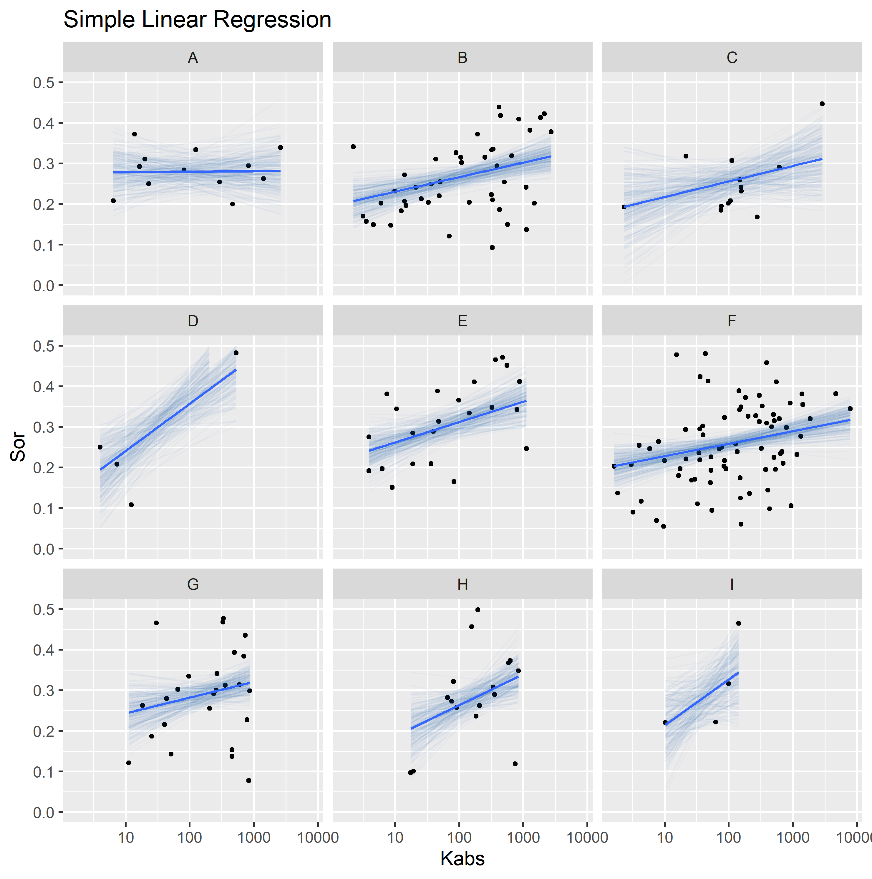
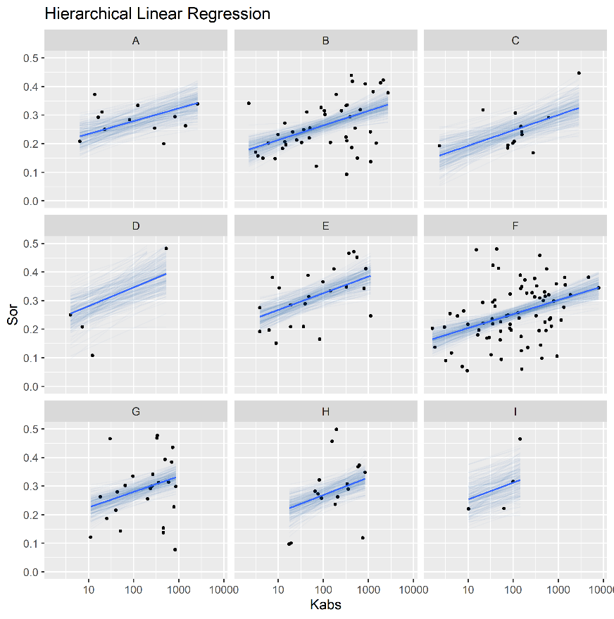
Figure 4.10: Simple (top) and Hierarchical (bottom) linear regression models of Sor vs log(kabs), grouped by reservoir.

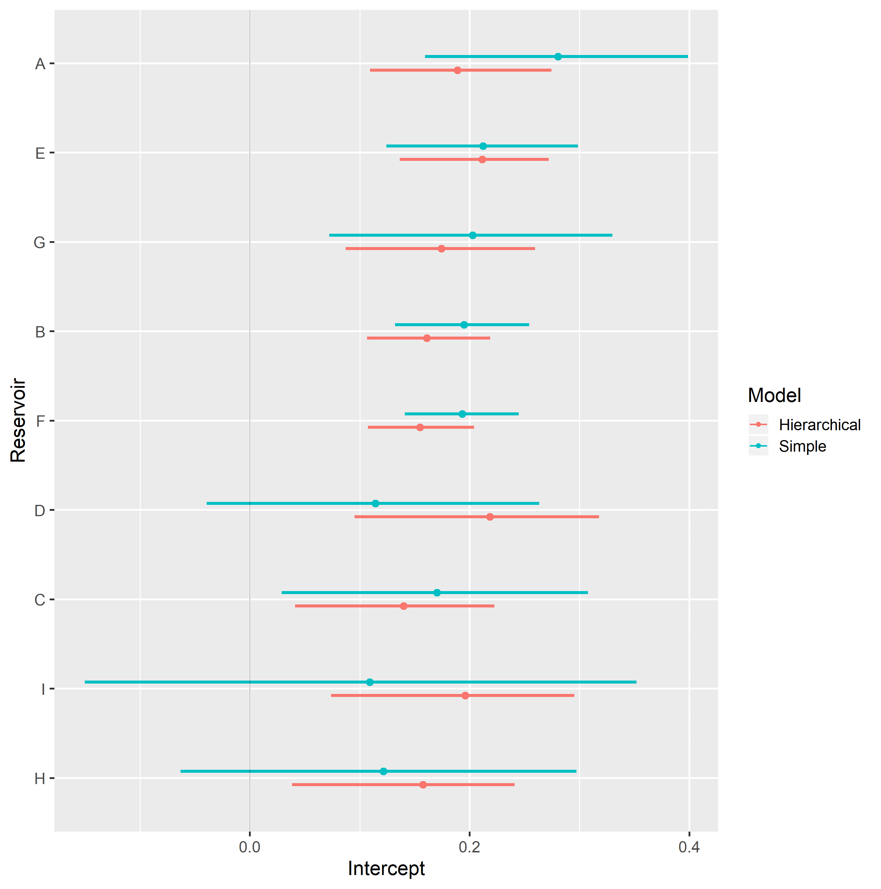
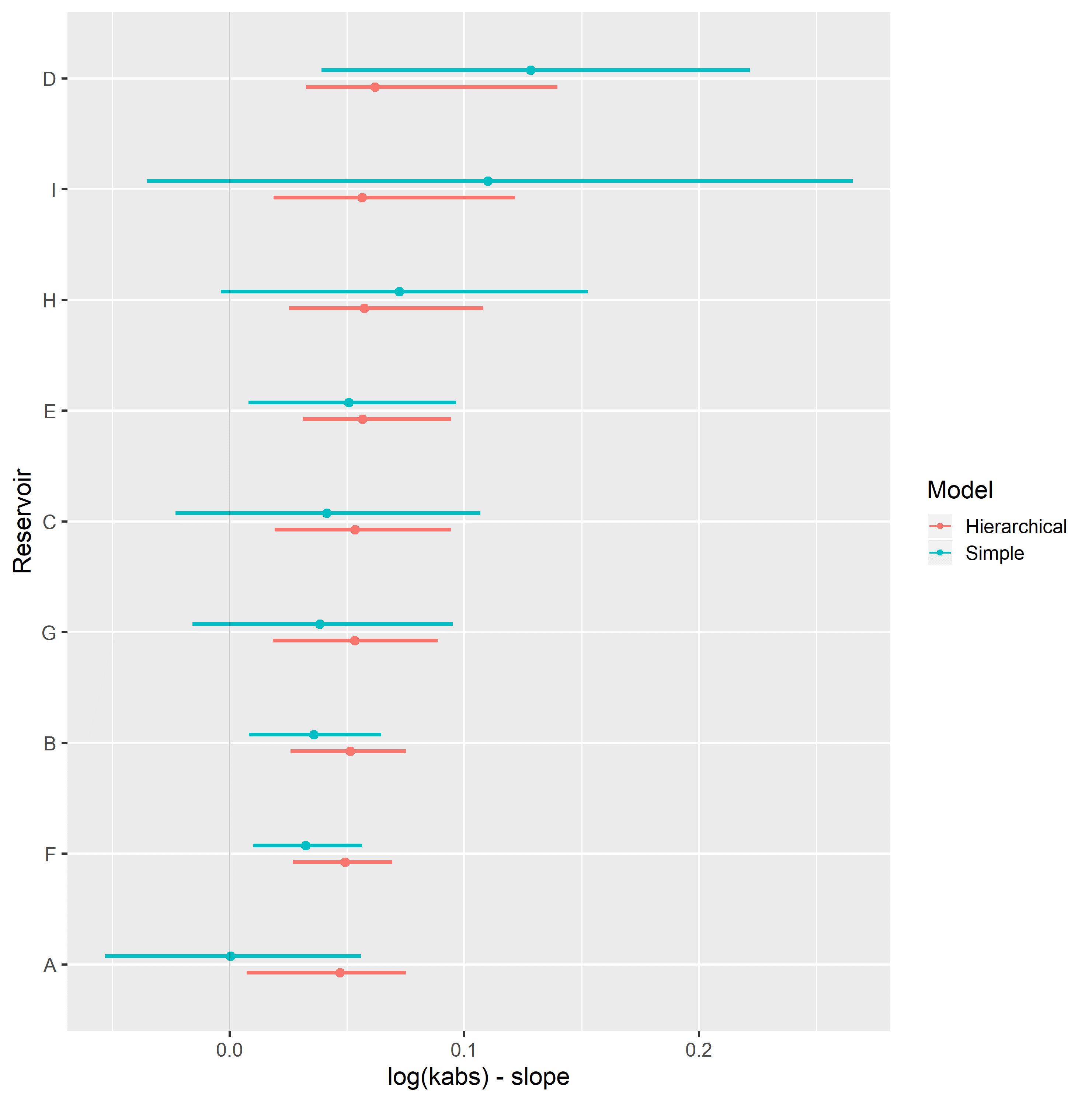
Figure 4.11: Intercept (top) and slope (bottom), simple and hierarchical linear regression Sor vs log(kabs) model parameters, grouped by reservoir.

Hierarchical varying slope and simple linear regression models of oil relative permeability at irreducible water saturation condition \(k_{ro}@S_{wi}\) and logarithm of absolute permeability \(\log{k_{abs}}\) were evaluated on the assembled dataset.

Table 4.3 displays the obtained regression metrics for each fitted model. Hierarchical linear regression achieved slightly better WAIC, LOOIC and \(R_{adj}^2\) metrics.

Table 4.3: \(k_{ro}@S_{wi}\) linear regression model metrics.

Regression Model	RMSE	WAIC	LOOIC	\(R^2\)	\(R_{adj}^2\)
Simple Linear Regression	0.20	-48.72	-47.50	0.34	0.28
Hierarchical Linear Regression	0.20	-62.02	-61.77	0.39	0.33

Figure 4.12 displays simple and hierarchical linear regression \(k_{ro}@S_{wi}\) vs \(\log{k_{abs}}\) models, grouped by reservoir. Black dots represent observed samples, light blue lines represent samples from the posterior distribution of intercept and slope parameters, and dark blue lines represent mean intercept and slope parameters, for each reservoir.

Completely pooled, simple linear regression models display larger between-groups slope variations and uncertainty, as shown in Figure 4.13. Reservoirs with large number of samples, such as reservoir F, show only small changes between hierarchical and simple linear regression model posterior distributions. A stronger regularizing effect is displayed in reservoir D, which contains a small number of samples. Overall behavior consistency of \(k_{ro}@S_{wi}\) in respect to \(\log{k_{abs}}\) is increased in the hierarchical partially pooled linear model, as slopes are regressed towards a common mean. As information is shared between different reservoirs, posterior uncertainties are noticeably reduced in the hierarchical linear model.

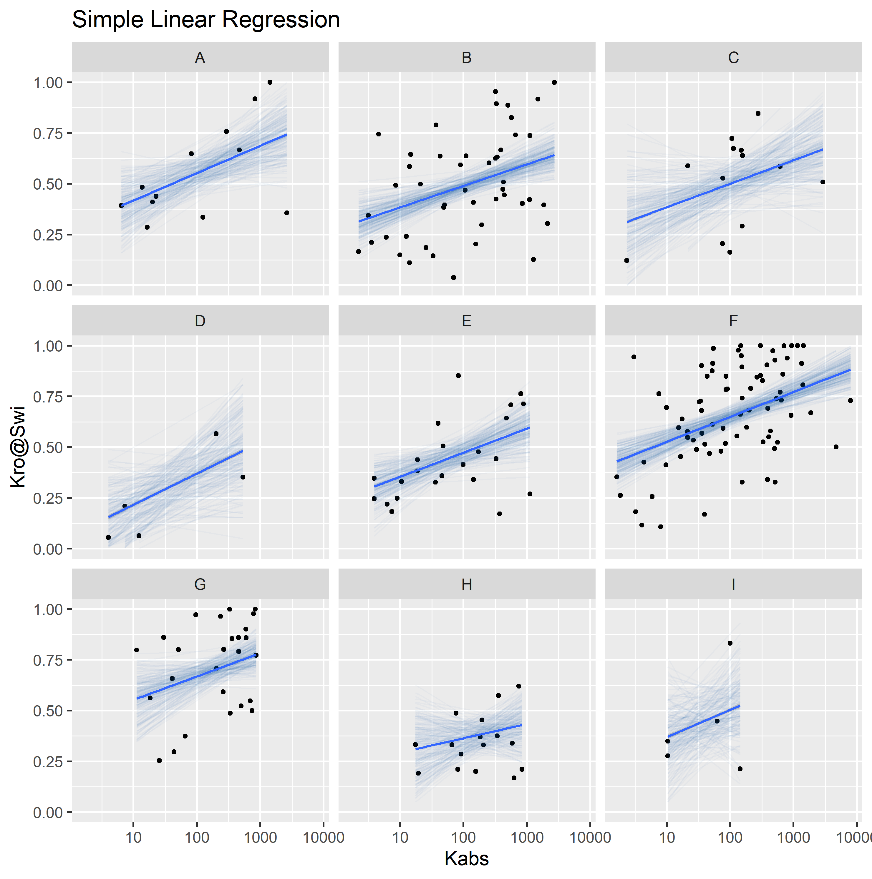
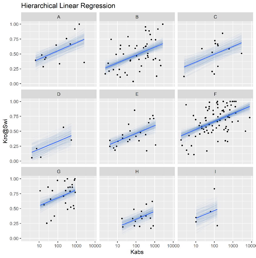
Figure 4.12: Simple (top) and Hierarchical (bottom) linear regression models of kro@Swi vs log(kabs), grouped by reservoir.

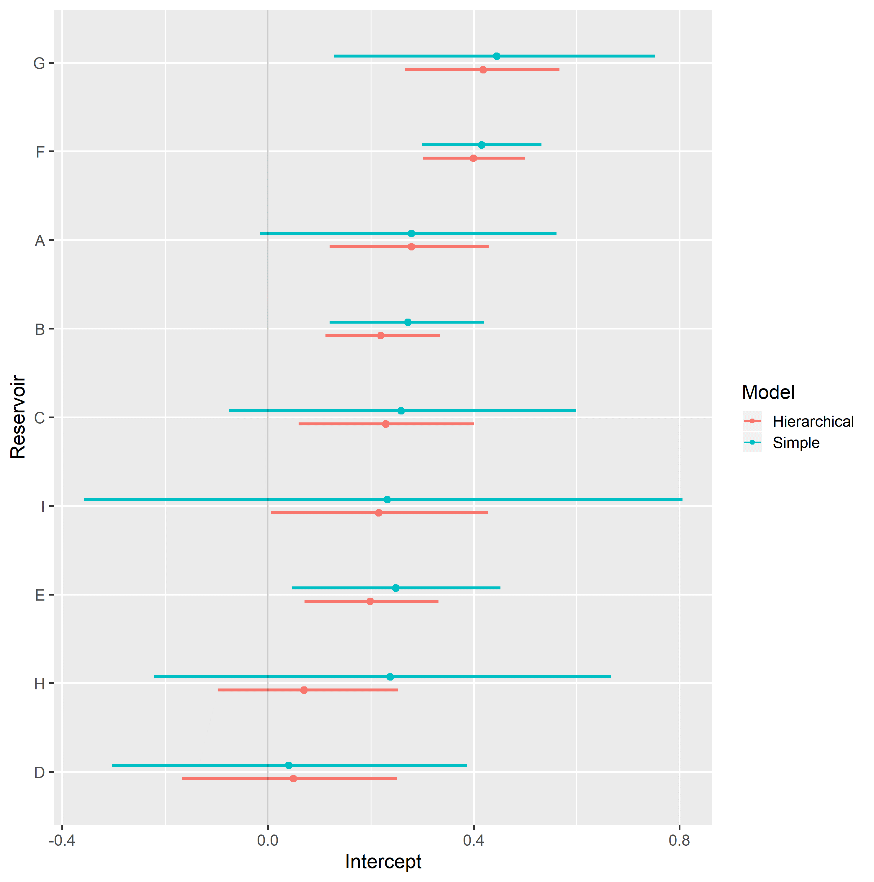
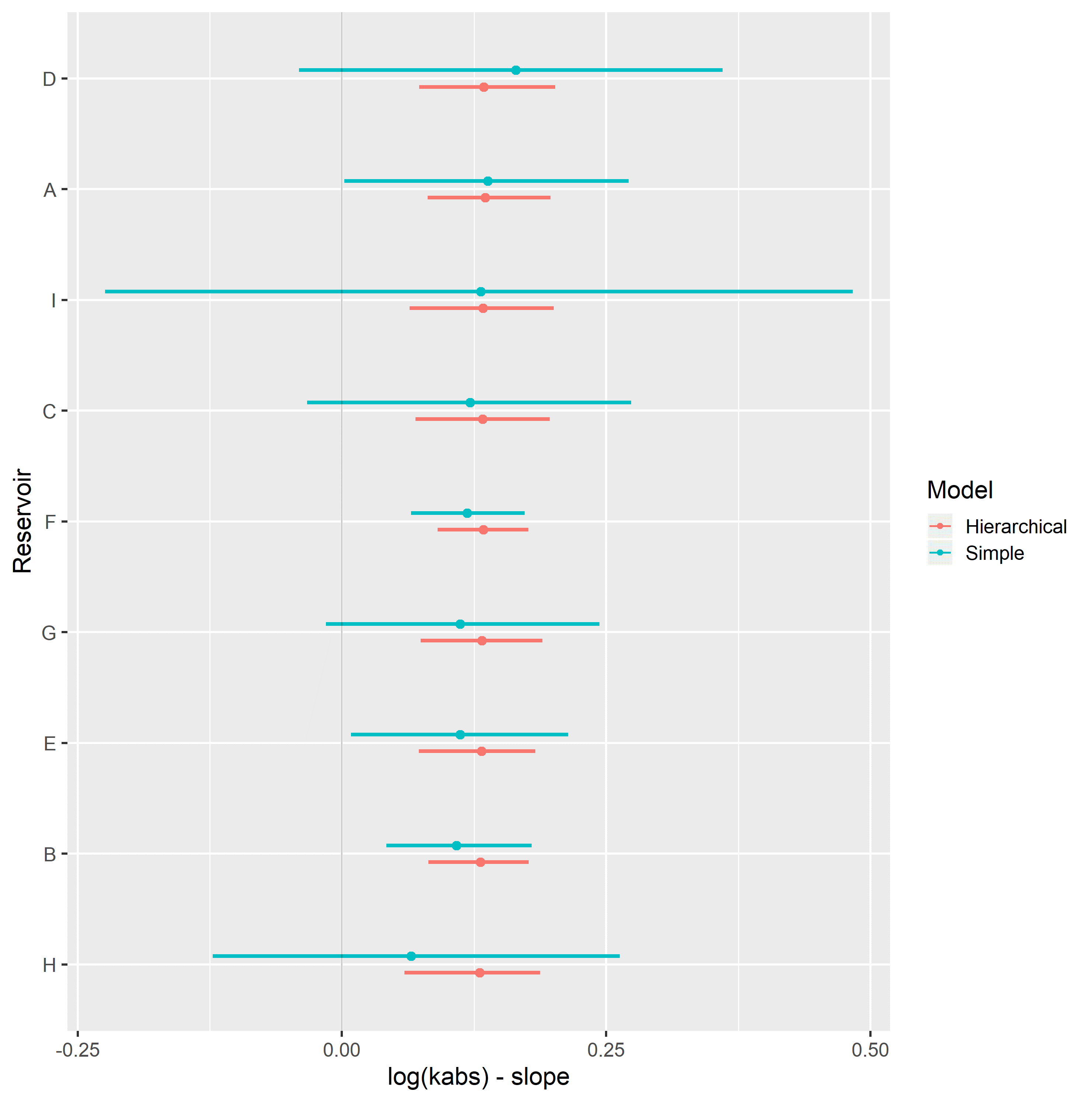
Figure 4.13: Intercept (top) and slope (bottom), simple and hierarchical linear regression kro@Swi vs log(kabs) model parameters, grouped by reservoir.

Hierarchical varying slope and simple linear regression models of water relative permeability at residual oil saturation condition \(k_{rw}@S_{or}\) and logarithm of absolute permeability \(\log{k_{abs}}\) were evaluated on the assembled dataset.

Table 4.4 displays the obtained regression metrics for each fitted model. Hierarchical linear regression achieved slightly better WAIC, LOOIC and \(R_{adj}^2\) metrics.

Table 4.4: \(k_{rw}@S_{or}\) linear regression model metrics.

Regression Model	RMSE	WAIC	LOOIC	\(R^2\)	\(R_{adj}^2\)
Simple Linear Regression	0.10	-366.62	-366.13	0.20	0.16
Hierarchical Linear Regression	0.10	-372.34	-372.18	0.24	0.17

Figure 4.14 displays simple and hierarchical linear regression \(k_{rw}@S_{or}\) vs \(\log{k_{abs}}\) models, grouped by reservoir. Black dots represent observed samples, light blue lines represent samples from the posterior distribution of intercept and slope parameters, and dark blue lines represent mean intercept and slope parameters, for each reservoir.

Completely pooled, simple linear regression models display larger between-groups slope variations and uncertainty, as shown in Figure 4.15. Reservoirs with large number of samples, such as reservoir F, show only small changes between hierarchical and simple linear regression model posterior distributions. A stronger regularizing effect is displayed in reservoir D, which contains a small number of samples. Overall behavior consistency of \(k_{rw}@S_{or}\) in respect to \(\log{k_{abs}}\) is increased in the hierarchical partially pooled linear model, as slopes are regressed towards a common mean. As information is shared between different reservoirs, posterior uncertainties are noticeably reduced in the hierarchical linear model.

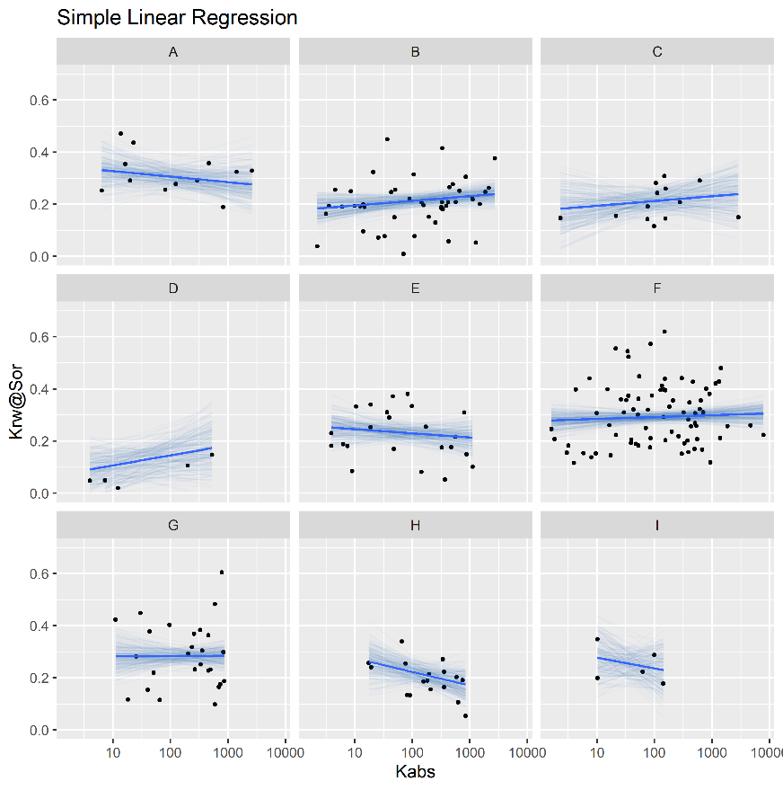
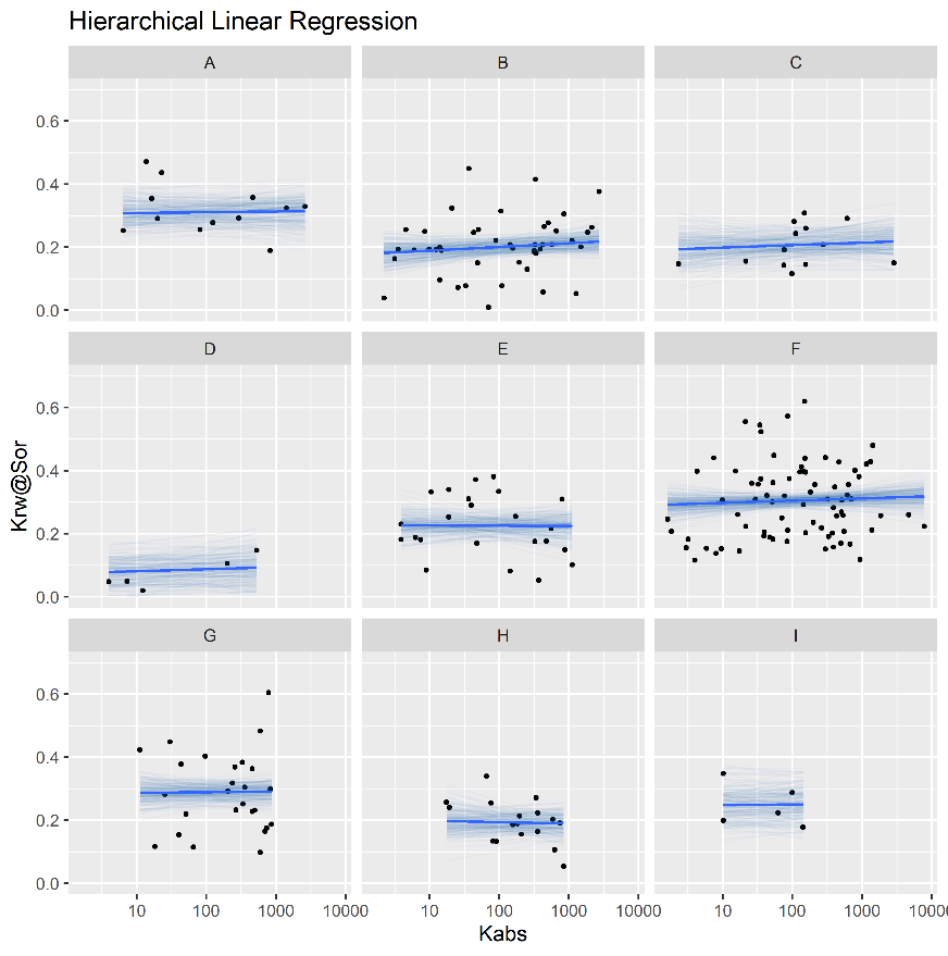
Figure 4.14: Simple (top) and Hierarchical (bottom) linear regression models of krw@Sor vs log(kabs), grouped by reservoir.

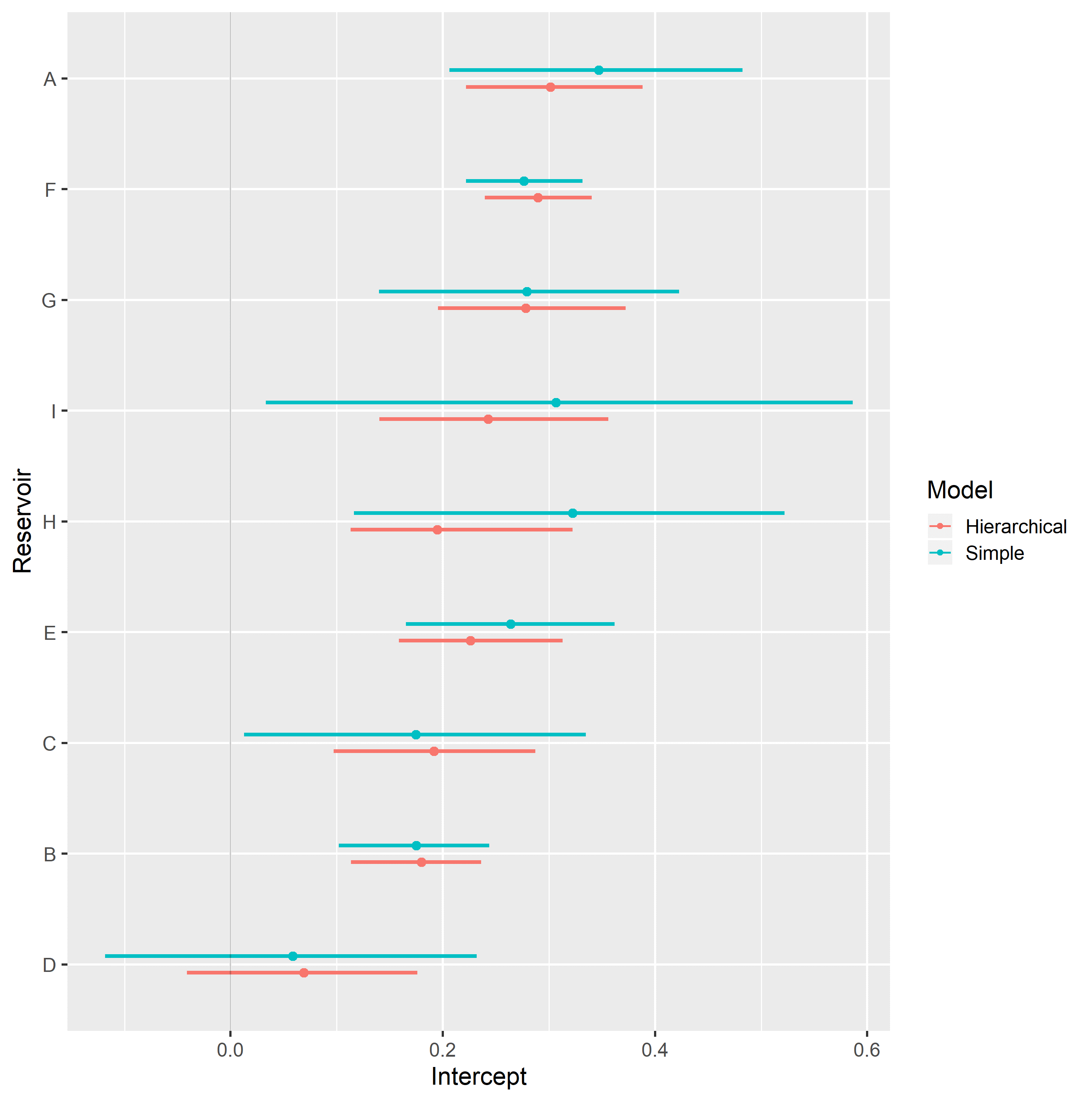
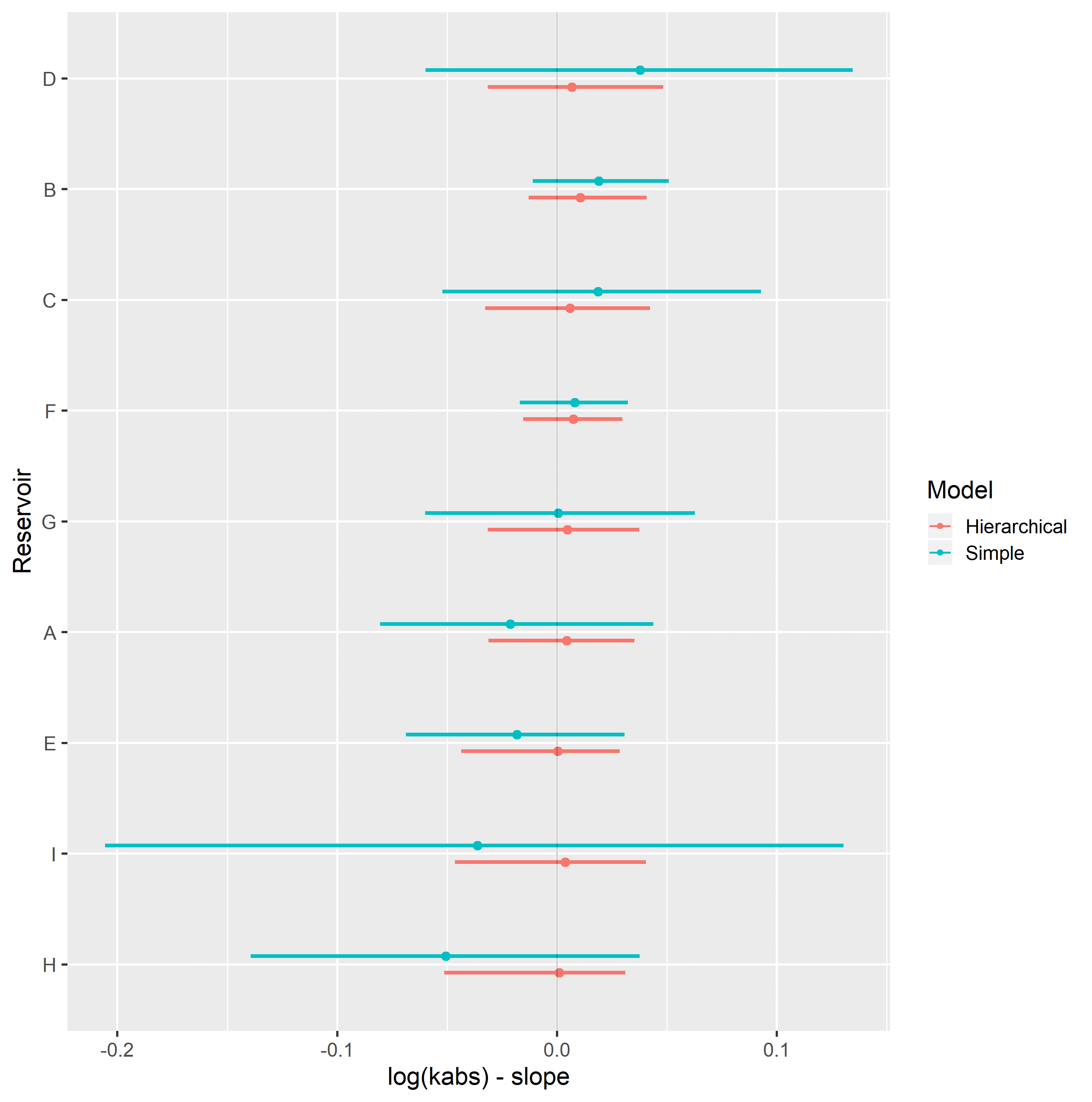
Figure 4.15: Intercept (top) and slope (bottom), simple and hierarchical linear regression krw@Sor vs log(kabs) model parameters, grouped by reservoir.

Posterior distribution of latent \(\mu_\alpha\) and \(\mu_\beta\) parameters of hierarchical linear regression models represent average behavior of model parameters across the different evaluated categories. Thus, they represent quantified petrophysical parameter model analogues, and may be used for preliminary characterization of reservoirs with similar characteristics as the ones used in the assembled model, but with no sampled data.

Multi-task simple and varying slopes hierarchical linear regression models, grouped by reservoir, were fitted to the assembled LET relative permeability parameter dataset. Comparison of WAIC and LOOIC metrics between them is shown in Table 4.5, displaying slightly better results for the multi-task hierarchical linear regression model.

Table 4.5: Multi-task linear regression model metrics.

Regression Model	WAIC	LOOIC
Simple Linear Regression	1119.6	1129.8
Hierarchical Linear Regression	1043.3	1048.0

The posterior distribution of the LET relative permeability parameters for a given reservoir and logarithmic absolute permeability may be used to sample relative permeability curves, fully incorporating the information from the available dataset, as exemplified in Figure 4.16.

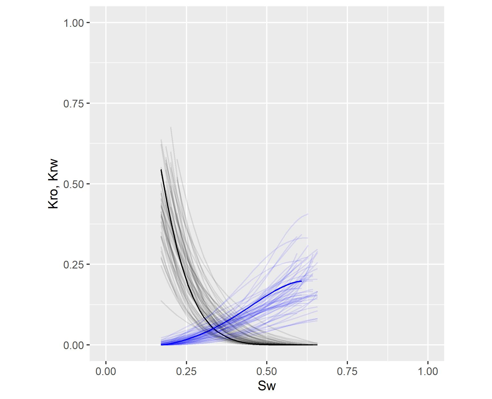
Figure 4.16: Example of multivariate posterior sample of relative permeability curves, fully incorporating the information from the available dataset.

References

Albuquerque, Marcelo R, Felipe M Eler, Heitor V R Camargo, André Compan, Dario Cruz, and Carlos Pedreira. 2018. “Estimation of Capillary Pressure Curves from Centrifuge Measurements using Inverse Methods.” Rio Oil & Gas Expo and Conference 2018,

Carpenter, Bob, Andrew Gelman, Matthew D. Hoffman, Daniel Lee, Ben Goodrich, Michael Betancourt, Marcus A. Brubaker, Jiqiang Guo, Peter Li, and Allen Riddell. 2017. “Stan: A probabilistic programming language.” Journal of Statistical Software 76 (1). https://doi.org/10.18637/jss.v076.i01.

DeGroot, Morris H., and Mark J. Schervish. 2012. Probability and Statistics. Edited by Addison-Wesley.

Gelman, Andrew, John B. Carlin, Hal S. Stern, David B. Dunson, Aki Vehtari, and Donald B. Rubin. 2014. Bayesian Data Analysis. 3. https://doi.org/10.1017/CBO9781107415324.004.

Gelman, Andrew, Ben Goodrich, Jonah Gabry, and Aki Vehtari. 2019. “R-Squared for Bayesian Regression Models.” The American Statistician 73 (3): 307–9.

Gelman, Andrew, Aleks Jakulin, Maria Grazia Pittau, and Yu Sung Su. 2008. “A weakly informative default prior distribution for logistic and other regression models.” Annals of Applied Statistics 2 (4): 1360–83. https://doi.org/10.1214/08-AOAS191.

Hoffman, Matthew D., and Andrew Gelman. 2014. “The no-U-turn sampler: Adaptively setting path lengths in Hamiltonian Monte Carlo.” Journal of Machine Learning Research 15: 1593–1623. http://arxiv.org/abs/1111.4246.

Lomeland, Frode, Einar Ebeltoft, and Wibeke Hammervold Thomas. 2005. “A new versatile relative permeability correlation.” International Symposium of the Society of Core Analysts, Toronto, Canada, 1–12.

Migon, Helio, Dani Gamerman, and Francisco Louzada. 2015. Statistical Inference. Second.

Peters, E. J. 2012. Advanced Petrophysics. Austin: Live Oak Book Company.

Vehtari, Aki, Andrew Gelman, and Jonah Gabry. 2017. “Practical Bayesian model evaluation using leave-one-out cross-validation and WAIC.” Statistics and Computing 27 (5): 1413–32. https://doi.org/10.1007/s11222-016-9696-4.